Dynamical analysis of a nonlocal delays spatial malaria model with Wolbachia-infected male mosquitoes release

Liping Wang; Runqi Liu; Yangyang Shi; Liping Wang; Runqi Liu; Yangyang Shi

doi:10.3934/era.2025139

Electronic Research Archive

2025, Volume 33, Issue 5: 3177-3200. doi: 10.3934/era.2025139

Previous Article Next Article

Research article

Dynamical analysis of a nonlocal delays spatial malaria model with Wolbachia-infected male mosquitoes release

1.
School of Mathematics-Physics and Finance, Anhui Polytechnic University, Wuhu 241000, China
2.
school of mathematics and information science, Shandong Technology and Business University, Yantai 264005, China

Received: 22 March 2025 Revised: 29 April 2025 Accepted: 08 May 2025 Published: 21 May 2025

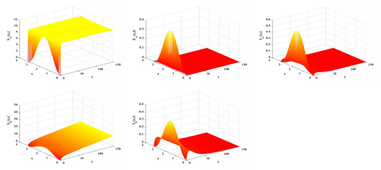
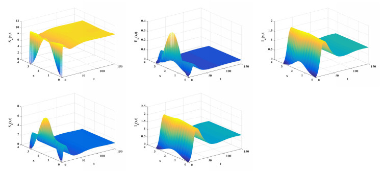
Malaria continues to pose a considerable threat to global health. This study investigates the use of releasing Wolbachia-infected male mosquitoes as a method to mitigate the spread of malaria. We have formulated a reaction-diffusion model with nonlocal delays that includes the Wolbachia release strategy. The basic reproduction number $ R_0 $ is defined within our model framework, serving as a critical threshold parameter that dictates the dynamic behavior of the model. A thorough dynamic analysis of the model reveals that when $ R_0 < 1 $, a globally attractive infection-free steady state is established. In contrast, if $ R_0 > 1 $, the disease persists uniformly. Numerical simulations are conducted to validate the theoretical results and to further illustrate the effectiveness of the Wolbachia release strategy on transmission and control of malaria. These simulations underscore the potential of using Wolbachia-infected male mosquitoes to significantly reduce spread of malaria.
- malaria,
- reaction-diffusion model,
- Wolbachia,
- nonlocal delays,
- basic reproduction number,
- dynamic analysis
Citation: Liping Wang, Runqi Liu, Yangyang Shi. Dynamical analysis of a nonlocal delays spatial malaria model with Wolbachia-infected male mosquitoes release[J]. Electronic Research Archive, 2025, 33(5): 3177-3200. doi: 10.3934/era.2025139

Related Papers:

Abstract

Malaria continues to pose a considerable threat to global health. This study investigates the use of releasing Wolbachia-infected male mosquitoes as a method to mitigate the spread of malaria. We have formulated a reaction-diffusion model with nonlocal delays that includes the Wolbachia release strategy. The basic reproduction number $ R_0 $ is defined within our model framework, serving as a critical threshold parameter that dictates the dynamic behavior of the model. A thorough dynamic analysis of the model reveals that when $ R_0 < 1 $, a globally attractive infection-free steady state is established. In contrast, if $ R_0 > 1 $, the disease persists uniformly. Numerical simulations are conducted to validate the theoretical results and to further illustrate the effectiveness of the Wolbachia release strategy on transmission and control of malaria. These simulations underscore the potential of using Wolbachia-infected male mosquitoes to significantly reduce spread of malaria.

References

[1]	N. J. White, S. Pukrittayakamee, Malaria, Lancet, 394 (2019), 1059–1070. https://doi.org/10.1016/S0140-6736(19)31752-7
[2]	Malaria, World Health Organization (WHO), 2024. Available from: https://www.who.int/news-room/fact-sheets/detail/malaria.
[3]	D. Lek, M. Shrestha, K. Lhazeen, T. Tobgyel, S. Kandel, G. Dahal, et al., Malaria elimination challenges in countries approaching the last mile: A discussion among regional stakeholders, Malaria J., 23 (2024), 401. https://doi.org/10.1186/s12936-024-05215-3 doi: 10.1186/s12936-024-05215-3
[4]	W. Wang, M. Zhou, X. Fan, T. Zhang, Global dynamics of a nonlocal PDE model for Lassa haemorrhagic fever transmission with periodic delays, Comput. Appl. Math., 43 (2024), 140. https://doi.org/10.1007/s40314-024-02662-1 doi: 10.1007/s40314-024-02662-1
[5]	W. Wang, X. Wang, X. Fan, Threshold dynamics of a reaction-advection-diffusion waterborne disease model with seasonality and human behavior change, Int. J. Biomath., 18 (2024), 2350106. https://doi.org/10.1142/S1793524523501061 doi: 10.1142/S1793524523501061
[6]	P. Wu, Global well-posedness and dynamics of spatial diffusion HIV model with CTLs response and chemotaxis, Math. Comput. Simul., 228 (2024), 402–417. https://doi.org/10.1016/j.matcom.2024.09.020 doi: 10.1016/j.matcom.2024.09.020
[7]	Y. Lou, X. Q. Zhao, A reaction-diffusion malaria model with incubation period in the vector population, J. Math. Biol., 62 (2011), 543–568. https://doi.org/10.1007/s00285-010-0346-8 doi: 10.1007/s00285-010-0346-8
[8]	Z. Bai, R. Peng, X. Q. Zhao, A reaction-diffusion malaria model with seasonality and incubation period, J. Math. Biol., 77 (2018), 201–228. https://doi.org/10.1007/s00285-017-1193-7 doi: 10.1007/s00285-017-1193-7
[9]	Z. Xu, On the global attractivity of a nonlocal and vector-bias malaria model, Appl. Math. Lett., 121 (2021), 107459. https://doi.org/10.1016/j.aml.2021.107459 doi: 10.1016/j.aml.2021.107459
[10]	B. He, Q. R. Wang, Threshold dynamics of a vector-bias malaria model with time-varying delays in environments of almost periodicity, Nonlinear Anal. Real World Appl., 78 (2024), 104078. https://doi.org/10.1016/j.nonrwa.2024.104078 doi: 10.1016/j.nonrwa.2024.104078
[11]	A. A. Hoffmann, B. L. Montgomery, J. Popovi$\acute{c}$, I. Iturbe-Ormaetxe, P. H. Johnson, F. Muzzi, et al., Successful establishment of Wolbachia in Aedes populations to suppress dengue transmission, Nature, 476 (2011), 454–457. https://doi.org/10.1038/nature10356 doi: 10.1038/nature10356
[12]	G. Bian, D. Joshi, Y. Dong, P. Lu, G. Zhou, X. Pan, et al., Wolbachia invades Anopheles stephensi populations and induces refractoriness to Plasmodium infection, Science, 340 (2013), 748–751. https://doi.org/10.1126/science.1236192 doi: 10.1126/science.1236192
[13]	C. L. Jeffries, G. G. Lawrence, G. Golovko, M. Kristan, J. Orsborne, K. Spence, et al., Novel Wolbachia strains in Anopheles malaria vectors from Sub-Saharan Africa, Wellcome Open Res., 3 (2018), 113. https://doi.org/10.12688/wellcomeopenres.14765.2 doi: 10.12688/wellcomeopenres.14765.2
[14]	G. L. Hughes, A. Rivero, J. L. Rasgon, Wolbachia can enhance Plasmodium infection in mosquitoes: Implications for malaria control?, PLoS Pathogens, 10 (2014), e1004182. https://doi.org/10.1371/journal.ppat.1004182 doi: 10.1371/journal.ppat.1004182
[15]	K. Liu, Y. Lou, A periodic delay differential system for mosquito control with Wolbachia incompatible insect technique, Nonlinear Anal. Real World Appl., 73 (2023), 103867. https://doi.org/10.1016/j.nonrwa.2023.103867 doi: 10.1016/j.nonrwa.2023.103867
[16]	J. Wu, Theory and Applications of Partial Functional Differential Equations, Springer, New York, 1996.
[17]	R. H. Martin, H. L. Smith, Abstract functional-differential equations and reaction-diffusion systems. Trans. Am. Math. Soc., 321 (1990), 1–44. https://doi.org/10.1090/S0002-9947-1990-0967316-X
[18]	J. K. Hale, Asymptotic behavior of dissipative systems, Am. Math. Soc., 25 (1988). https://dhttp://dx.doi.org/10.1090/surv/025
[19]	Y. Zha, W. Jiang, Transmission dynamics of a reaction-advection-diffusion dengue fever model with seasonal developmental durations and intrinsic incubation periods, J. Math. Biol., 88 (2024), 74. https://doi.org/10.1007/s00285-024-02089-6 doi: 10.1007/s00285-024-02089-6
[20]	L. Zhang, Z. Wang, X. Q. Zhao, Threshold dynamics of a time periodic reaction-diffusion epidemic model with latent period, J. Differ. Equations, 258 (2015), 3011–3036. https://doi.org/10.1016/j.jde.2014.12.032 doi: 10.1016/j.jde.2014.12.032
[21]	H. L. Smith, Monotone Dynamical Systems: An Introduction to the Theory of Competitive and Cooperative Systems, American Mathematical Society, Providence, 2008.
[22]	W. Wang, X. Zhao, A nonlocal and time-delayed reaction-diffusion model of dengue transmission, SIAM J. Appl. Math., 71 (2011), 147–168. https://doi.org/10.1137/090775890 doi: 10.1137/090775890
[23]	H. R. Thieme, Spectral bound and reproduction number for infinite-dimensional population structure and time heterogeneity, SIAM J. Appl. Math., 70 (2009), 188–211. https://doi.org/10.1137/080732870 doi: 10.1137/080732870
[24]	H. L. Smith, X. Q. Zhao, Robust persistence for semidynamical systems, Nonlinear Anal., 47 (2001), 6169–6179. https://doi.org/10.1016/S0362-546X(01)00678-2 doi: 10.1016/S0362-546X(01)00678-2
[25]	R. Wu, X. Q. Zhao, A reaction-diffusion model of vector-borne disease with periodic delays, J. Nonlinear Sci., 29 (2019), 29–64. https://doi.org/10.1007/s00332-018-9475-9 doi: 10.1007/s00332-018-9475-9
[26]	W. Wang, X. Q. Zhao, Basic reproduction numbers for reaction-diffusion epidemic models, SIAM J. Appl. Dyn. Syst., 11 (2012), 1652–1673. https://doi.org/10.1137/120872942 doi: 10.1137/120872942

Reader Comments

Your name:*

Email:*
© 2025 the Author(s), licensee AIMS Press. This is an open access article distributed under the terms of the Creative Commons Attribution License (http://creativecommons.org/licenses/by/4.0)