Modeling the variable transmission rate and various discharges on the spread of Malaria

Jitendra Singh; Maninder Singh Arora; Sunil Sharma; Jang B. Shukla; Jitendra Singh; Maninder Singh Arora; Sunil Sharma; Jang B. Shukla

doi:10.3934/era.2023016

Electronic Research Archive

2023, Volume 31, Issue 1: 319-341. doi: 10.3934/era.2023016

Previous Article Next Article

Research article

Modeling the variable transmission rate and various discharges on the spread of Malaria

1.
PPN College, CSJM University, Kanpur 208001, India
2.
Department of Information System, College of Computer and Information Sciences, Majmaah University, Majmaah 11952, Saudi Arabia
3.
International Internet University for Research in Science and Technology, Kanpur 208017, India

Academic Editor: Lixia Duan

Received: 15 August 2022 Revised: 10 October 2022 Accepted: 17 October 2022 Published: 01 November 2022

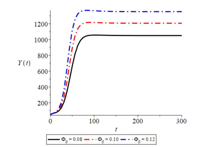
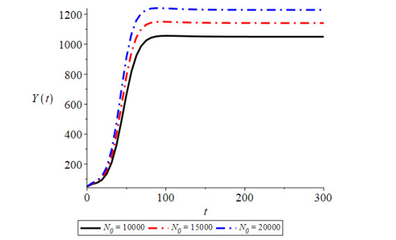
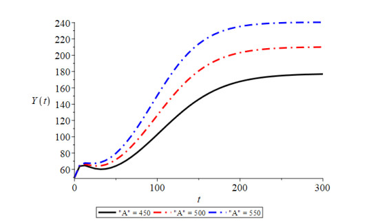
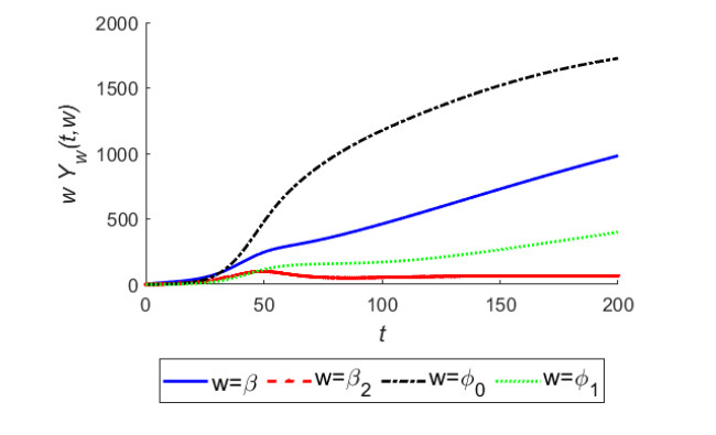
Natural and household discharges are the natural breeding grounds of various mosquito species, including female Anopheles mosquitoes, which transmit the Plasmodium parasite, causing the spread of the life-threatening disease malaria. Apart from that, population migrations also have a substantial impact on malaria transmission, claiming about half a million lives every year around the world. To assess the effects of the cumulative density of households and other natural discharges, and emigration-dependent interaction rates on the dissemination of the vector-borne infectious disease malaria, we propose and analyze a non-linear mathematical model. The model comprises five dependent variables, namely, the density of the susceptible human population, the density of the infective human population, the density of the susceptible female Anopheles mosquito population, the density of the infective mosquito population and cumulative density of household and other natural discharges. In the model, the density of the mosquito population is supposed to follow logistic growth, whose intrinsic growth rate is a linear function of the cumulative density of household and other natural discharges. The nonlinear model is analyzed by using the stability theory of differential equations, numerical simulations and sensitivity analysis. The analysis shows that an increase in non-emigrating population causes increased incidence of malaria. It is also found that an increase in household and other natural discharges accelerates the occurrence of malaria. A basic differential sensitivity analysis is carried out to assess the sensitivity of model solutions with respect to key parameters. The model's numerical simulations demonstrate the analytical findings.
- infectious disease,
- Malaria,
- emigration,
- stability
Citation: Jitendra Singh, Maninder Singh Arora, Sunil Sharma, Jang B. Shukla. Modeling the variable transmission rate and various discharges on the spread of Malaria[J]. Electronic Research Archive, 2023, 31(1): 319-341. doi: 10.3934/era.2023016

Related Papers:

Abstract

Natural and household discharges are the natural breeding grounds of various mosquito species, including female Anopheles mosquitoes, which transmit the Plasmodium parasite, causing the spread of the life-threatening disease malaria. Apart from that, population migrations also have a substantial impact on malaria transmission, claiming about half a million lives every year around the world. To assess the effects of the cumulative density of households and other natural discharges, and emigration-dependent interaction rates on the dissemination of the vector-borne infectious disease malaria, we propose and analyze a non-linear mathematical model. The model comprises five dependent variables, namely, the density of the susceptible human population, the density of the infective human population, the density of the susceptible female Anopheles mosquito population, the density of the infective mosquito population and cumulative density of household and other natural discharges. In the model, the density of the mosquito population is supposed to follow logistic growth, whose intrinsic growth rate is a linear function of the cumulative density of household and other natural discharges. The nonlinear model is analyzed by using the stability theory of differential equations, numerical simulations and sensitivity analysis. The analysis shows that an increase in non-emigrating population causes increased incidence of malaria. It is also found that an increase in household and other natural discharges accelerates the occurrence of malaria. A basic differential sensitivity analysis is carried out to assess the sensitivity of model solutions with respect to key parameters. The model's numerical simulations demonstrate the analytical findings.

References

[1]	WHO Malaria: Fact sheets, 2022. Available from: https://www.who.int/news-room/fact-sheets/detail/malaria.
[2]	S. Sato, Plasmodium-a brief introduction to the parasites causing human malaria and their basic biology, J. Physiol. Anthropol., 40 (2021), 1–13. https://doi.org/10.1186/s40101-020-00251-9 doi: 10.1186/s40101-020-00251-9
[3]	E. Pondeville, N. Puchot, M. Lang, F. Cherrier, F. Schaffner, C. Dauphin-Villemant, et al., Evolution of sexually-transferred steroids and mating-induced phenotypes in Anopheles mosquitoes, Sci. Rep., 9 (2019), 4669. https://doi.org/10.1038/s41598-019-41094-4 doi: 10.1038/s41598-019-41094-4
[4]	N. T. J. Bailey, The Biomathematics of Malaria, Charles Griffin & Company Ltd., 1982.
[5]	L. Cai, Z. Li, C. Yang, J. Wang, Global analysis of an environmental disease transmission model linking within-host and between-host dynamics, Appl. Math. Model., 86 (2020), 404–423. https://doi.org/10.1016/j.apm.2020.05.022 doi: 10.1016/j.apm.2020.05.022
[6]	F. Brauer, C. Castillo-Chavez, Z. Feng, Mathematical Models in Epidemiology, Springer, New York, 2019.
[7]	M. Ghosh, P. Chandra, P. Sinha, J. B. Shukla, Modelling the carrier dependent infectious diseases with environmental effects, Appl. Math. Comput., 157 (2004), 385–402. https://doi.org/10.1016/S0096-3003(03)00564-2 doi: 10.1016/S0096-3003(03)00564-2
[8]	D. J. Rogers, S. E. Randolph, The global spread of malaria in a future warmer world, Science, 289 (2000), 1763–1766. https://doi.org/10.1126/science.289.5485.176 doi: 10.1126/science.289.5485.176
[9]	C. L. Mitchell, M. M. Janko, M. K. Mwandagalirwa, A. K. Tshefu, J. K. Edwards, B. W. Pence, et al., Impact of extractive industries on malaria prevalence in the Democratic Republic of the Congo: a population-based cross-sectional study, Sci. Rep., 12 (2022), 1–9.
[10]	F. J. Colón-González, M. O. Sewe, A. M. Tompkins, H. Sjödin, A. Casallas, J. Rocklöv, et al., Projecting the risk of mosquito-borne diseases in a warmer and more populated world: a multi-model, multi-scenario intercomparison modelling study, Lancet Planet. Health, 5 (2021), 404–414. https://doi.org/10.1016/S2542-5196(21)00132-7 doi: 10.1016/S2542-5196(21)00132-7
[11]	R. M. Anderson, R. M. May, Infectious Diseases of Humans: Dynamics and Control, Oxford University Press, London, U.K., 1991.
[12]	M. S. Arora, S. Singh, A. Omar, A. Malviya, J. B. Shukla, Effect of global warming temperature on the spread of bacteria dependent infectious diseases, Int. J. Clim. Change: Impacts Responses, 13 (2021), 1–19. https://doi.org/10.18848/1835-7156/CGP/v13i02/1-19 doi: 10.18848/1835-7156/CGP/v13i02/1-19
[13]	J. B. Shukla, V. Singh, A. K. Mishra, Modeling the spread of an infectious disease with bacteria and carriers in the environment, Nonlinear Anal.: Real World Appl., 12 (2011), 2541–2551. https://doi.org/10.1016/j.nonrwa.2011.03.003 doi: 10.1016/j.nonrwa.2011.03.003
[14]	S. Singh, Modeling the effect of global warming on the spread of carrier dependent infectious diseases, Model. Earth. Syst. Environ., 3 (2017), 3–39. https://doi.org/10.1007/s40808-017-0272-5 doi: 10.1007/s40808-017-0272-5
[15]	S. Singh, A. Omar, A. Modelling and analysis the effect of global warming on the spread of carrier dependent infectious diseases, Jnanabha, 50 (2020), 189–206.
[16]	A. ul Rehman, R. Singh, T. Abdeljawad, E. Okyere, L. Guran, Modeling, analysis and numerical solution to malaria fractional model with temporary immunity and relapse, Adv. Differ. Equations, 390 (2021). https://doi.org/10.1186/s13662-021-03532-4
[17]	S. Singh, J. B. Shukla, P. Chandra, Modelling and analysis of the spread of malaria: Environmental and ecological effects, J. Biol. Syst., 13 (2005), 1–11. https://doi.org/10.1142/S0218339005001367 doi: 10.1142/S0218339005001367
[18]	M. Ghosh, A. A. Lashari, X. Li, Biological control of malaria: A mathematical model, Appl. Math. Comput., 219 (2013), 7923–7939. https://doi.org/10.1016/j.amc.2013.02.053 doi: 10.1016/j.amc.2013.02.053
[19]	E. Ndamuzi, P. Gahungu, Mathematical modeling of Malaria transmission dynamics: Case of burundi, J. Appl. Math. Phys., 9 (2021), 2447–2460. https://doi.org/10.4236/jamp.2021.910156 doi: 10.4236/jamp.2021.910156
[20]	H. Wu, Z. Hu, Malaria transmission model with transmission-blocking drugs and a time delay, Math. Probl. Eng., (2021), 1–17. https://doi.org/10.1155/2021/1339086
[21]	B. Traoré, O. Koutou, B. Sangaré, A global mathematical model of malaria transmission dynamics with structured mosquito population and temperature variations, Nonlinear Anal.: Real World Appl., 53 (2020). https://doi.org/10.1016/j.nonrwa.2019.103081
[22]	A. Elaiw, A. A. Agha, Global analysis of a reaction-diffusion within-host Malaria infection model with adaptive immune response, Mathematics, 8 (2020), 563. https://doi.org/10.3390/math8040563 doi: 10.3390/math8040563
[23]	S. Noeiaghdam, A. Dreglea, H. Işık, M. Suleman, A comparative study between discrete stochastic arithmetic and floating-point arithmetic to validate the results of fractional order model of Malaria infection, Mathematics, 9 (2021), 1435. https://doi.org/10.3390/math9121435 doi: 10.3390/math9121435
[24]	S. Noeiaghdam, S. Micula, Dynamical strategy to control the accuracy of the nonlinear bio-mathematical model of Malaria infection, Mathematics, 9 (2021), 1031. https://doi.org/10.3390/math9091031 doi: 10.3390/math9091031
[25]	S. Singh, J. Singh, J. B. Shukla, Modelling and analysis of the effects of density dependent contact rates on the spread of carrier dependent infectious diseases with environmental discharges, Model. Earth Syst. Environ., 5 (2019), 21–32. https://doi.org/10.1007/s40808-018-0515-0 doi: 10.1007/s40808-018-0515-0
[26]	S. Tang, L. Chen, Density-dependent birth rate, birth pulses and their population dynamic consequences, J. Math. Biol., 44 (2002), 185–199. https://doi.org/10.1007/s002850100121 doi: 10.1007/s002850100121
[27]	H. W. Hethcote, Q. Linda, Disease transmission models with density-dependent demographics, Math. Biosci., 128 (1992), 93–130. https://doi.org/10.3817/0992093130 doi: 10.3817/0992093130
[28]	S. Singh, J. Singh, S. K. Sharma, J. B. Shukla, The effect of density dependent emigration on spread of infectious diseases: a modelling study, Rev. Latinoam. Hipertens., 14 (2019), 83–88.
[29]	J. Zhou, H. W. Hethcote, Population size dependent incidence in models for diseases without immunity, J. Math. Biol., 32 (1994), 809–834. https://doi.org/10.1007/BF00168799 doi: 10.1007/BF00168799
[30]	J. B. Shukla, S. Singh, J. Singh, S. K. Sharma, Modelling and analysis of bacteria dependent infectious diseases with variable contact rates, Comput. Materals Contin., 68 (2021), 1859–1875. https://doi.org/10.32604/cmc.2021.012095 doi: 10.32604/cmc.2021.012095
[31]	H. W. Hethcote, Qualitative analyses of communicable disease models, Math. Biosci., 28 (1976), 335–356. https://doi.org/10.1016/0025-5564(76)90132-2 doi: 10.1016/0025-5564(76)90132-2
[32]	D. Greenhalgh, Some threshold and stability results for epidemic models with a density dependent death rate, Theor. Popul. Biol., 42 (1990), 130–151. https://doi.org/10.1016/0040-5809(92)90009-I doi: 10.1016/0040-5809(92)90009-I
[33]	D. M. Bortz, P. W. Nelson, Sensitivity analysis of a nonlinear lumped parameter model of HIV infection dynamics, Bull. Math. Biol., 66 (2004), 1009–1026. https://doi.org/10.1016/j.bulm.2003.10.011 doi: 10.1016/j.bulm.2003.10.011

Reader Comments

Your name:*

Email:*
© 2023 the Author(s), licensee AIMS Press. This is an open access article distributed under the terms of the Creative Commons Attribution License (http://creativecommons.org/licenses/by/4.0)