Dynamics of a stochastic epidemic model with information intervention and vertical transmission

1.   Introduction

Outbreaks of infectious diseases do great harm to life and fortune. The construction and research of mathematical models play an extremely important role in the prevention and control of diseases. Scholars have studied various properties of many epidemic models, such as SIR (Susceptible-Infected-Recovered), SEIR (Susceptible-Exposed-Infected-Recovered), SIRS, SIQS (Susceptible-Infected-Quarantined-Recovered), which portray different characteristics of disease transmission^{[1,2,3,4,5,6]}. The authors in ^[6] studied the Hopf bifurcation and stability of a delayed SIR model. They established an epidemic model with temporary immunity and specific functional response^[7], and got the well-possedness and the threshold to determine different behaviors of the model.

When an epidemic occurs, people can learn about the transmission route of the disease, prevention measures and the government's policy on disease control from media such as the TV or Internet, so that they can take certain measures to slow down the spread of the disease, such as self-isolation, vaccination, and compliance with the government's anti-epidemic regulations. On account of the role of media information on disease control, scholars have studied the different properties of epidemic models with information intervention^{[8,9,10,11,12]}. At present, there are mainly two ways to study the impact of information intervention on the behavior. One is to study the impact of information intervention on the contact rate^[8,9,13,14], and the other is to introduce a new class with information awareness^{[10,11,15,16]}. In ^[15], the following epidemic model with separate information intervention class was established:

where $S_t$, $I_t$, $R_t$ denote the quantity of the susceptible class, the infected class, and the recovered class at time $t$, separately. $M_t$ represents the individuals of the class with information awareness. The meanings of the parameters in model (1.1) are shown in Table 1. In addition, $a_2$ represents the degradation rate of information, which contains the subtraction due to the natural death of $M$. Thus, the assumption that $a_2 > d_1$ is reasonable. The whole part $d_2m$ indicates response rate; the detailed meaning of each parameter on the information and schematic diagram of the above model can be seen in ^[15]. All the above parameters are specified as positive.

Reality is not immutable and often full of various uncertainties. The above deterministic model (1.1) can not reflect these uncertain factors. Therefore, the introduction of the model with stochastic noise will better reflect the reality and present more research contexts. For this reason, many scholars have studied epidemic models with various stochastic factors^{[17,18,19,20]}. The authors have studied the nontrivial positive periodic solution and condition for extinction of the model with media coverage and white noise^[18]. Bao-Shao investigated an SIRS model with Markovian switching, which is used to describe the changes of coefficients in different environments, and discussed the influence of Markovian switching on the behavior of the model. In this paper, we introduce the stochastic perturbation of white noise into the above model, whose intensity is proportional to each class, that is

Here, $W_i(t), i = 1, 2, 3, 4$ are mutually independent Brownian motions on probability space and $\sigma_i, i = 1, 2, 3, 4$ represent the intensities of the stochastic perturbations. The greater the stochastic perturbations, the deeper the impact on the system, the greater $\sigma_i$ will be.

In addition to physical or respiratory transmission, there is also a form of vertical transmission from an infected mother to the newborns, such as with hepatitis B and AIDS. Vertical transmission from the mother to the newborn is considered as one of the most important ways of AIDS transmission. Thus, the epidemic models possessing vertical transmission have been extensively investigated^[21,22,23]. The authors in ^[21] proposed an epidemic model with vertical transmission where the parameter $b$ signifies the birth rate of the population and $q$ stands for the proportion of newborns infected after birth from infectious mothers. $p = 1-q$ and $d_1 > b\ge 0$ is assumed. Therefore, $pb$ expresses the rate of newborns who have not been infected by their mothers and become susceptible.

Hence, introducing the above factors, including the information intervention and vertical transmission, we can obtain the following stochastic model:

The above factors not only make the model more general, but also raise the degree of difficulty of the study. The novelties of this paper are as follows: (ⅰ) An epidemic model with information intervention and vertical transmission is established; (ⅱ) a threshold is obtained to determine the different dynamics of the model and the exponential rates of three classes are studied; (ⅲ) the critical case of $\Delta = 0$, which has rarely been discussed in the literature, is investigated here.

This paper is arranged as follows: In Section 2, some estimations of the solution are given, followed by some lemmas to be used later. Section 3 gives a rough illustration of the value for disease extinction and provides the main conclusions of the paper. Part 4 focuses on the proof of Theorem 3.1 and Proposition 3.1 in detail. Part 5 proves the persistence of the model when $\Delta > 0$ and obtains the condition that the model has a stationary distribution. Section 6 studies the critical case when $\Delta = 0$. Section 7 discusses the results of the paper and lists some examples and numerical simulations to check the previous results.

2.   Background knowledge

In this paper, $(\Omega, \mathfrak{F}, \{\mathfrak{F}\}_t, \mathbb{P})$ is assumed to be a complete probability space and $\mathbb{R}_+^4: = \{(a, b, c, d)|a\ge0, b\ge0, c\ge0, d\ge0\}$ and $\mathbb{R}_+^{4, o}: = \{(a, b, c, d)|a > 0, b > 0, c > 0, d > 0\}$. $a\wedge b = \min\{a, b\}$. $\mathbb{P}_{s, i, m_0, r}$ and $\mathbb{E}_{s, i, m_0, r}$ denote the probability and expectation with initial condition $(s, i, m_0, r)$, respectively.

For the general SDE $dx_t = f(x_t)dt+g(x_t)dW(t)$ and the twice-differentiable function $V(x)$, the operator $\mathcal{L}V$ is defined by

In addition, the $\rm It\hat{o}'s$ formula can be expressed as

First of all, we are concerned with the existence and uniqueness as well as approximate scope of the solution. The following lemmas will respond to these problems.

Lemma 2.1.

(i) For the initial condition $(s, i, m_0, r)\in \mathbb{R}_+^4$, the model (1.3) has a global solution $(S_t, I_t, M_t, R_t)$ that possesses Markov-Feller property. Moreover, the solution $(S_t, I_t, M_t, R_t)$ will remain in $\mathbb{R}_+^4$ with probability 1.

(ii) Let $\sigma = \max\{\sigma_1, \sigma_2, \sigma_3, \sigma_4\}$, for $0 < \vartheta < p < \theta < \frac{2(d_1-b)}{\sigma^2}$, there exist constants $N_1 > 0$ and $N_2 > 0$ satisfying

Proof. The proof of part (ⅰ) is common and omitted. Our main proof is part (ⅱ). Let $V_1(S, I, M, R): = (S+I+M+R)^{1+\theta}+S^{-\vartheta}$. Direct calculation to $V_1(S, I, M, R)$ yields to

Let $0 < \vartheta < p < \theta < \frac{2(d_1-b)}{\sigma^2}$, so $\frac{\vartheta(1+p)}{p} < 1+\vartheta$ and $-(d_1-b)+\frac{\theta\sigma^2}{2} < 0$ hold true. By using Young's inequality, it has

and

Hence,

Let $N_1 = d_1-b-\frac{\theta\sigma^2}{2}$, then $\mathcal{L}V_1(S, I, M, R)+N_1V_1(S, I, M, R)\leq N_2$, where

The rest of the process is standard; one can see Lemma 2.3 in ^[24]. Thus, (2.3) is obtained. □

Lemma 2.2. For all initial conditions $(s, i, m_0, r)\in \mathbb{R}_+^4$, the solution $(S_t, I_t, M_t, R_t)$ of (1.3) satisfies

hence,

Moreover, it has

Proof. For (2.4), the proof is analogous to Lemma 3.1 in ^[22], mainly utilizing the result of Theorem 3.9 in ^[25], so it is omitted here. The proofs for (2.5) can be derived from (2.4) and strong law of large numbers.

For $\lim_{t\to\infty}\frac{\ln S_t}{t}\leq0$ and other formulas in (2.6), we recommend Lemma 2.3 in ^[26] to get a detailed proof. In addition, the property that $\mathbb{E}S_t^{-\vartheta} < \infty$ will lead to $\liminf_{t\to\infty}\frac{\ln S_t}{t}\ge0$, so $\lim_{t\to\infty}\frac{\ln S_t}{t} = 0$ is obtained.

□

3.   The threshold to determine the extinction or permanence of model (1.3)

We will give a value in this section and roughly explain it as the threshold of the extinction or persistence of model (1.3).

Take into account the first equation of model (1.3) on the boundary $I_t = 0$, $M_t = 0$, and $R_t = 0$, it has

Let $\bar{S}^u_t$ be the solution to (3.1) with the initial condition $\bar{S}_0 = u$. It should be noted that $S_t\leq\bar{S}_t, \; t > 0$ cannot be obtained by using the comparison theorem. Applying the $\rm It\hat{o}'s$ formula to the function $\bar{S}-1-\ln \bar{S}$ and making use of the result in ^[27], there exists the unique stationary distribution $\pi_0$ for (3.1) with the density

where $\bar{v} = \frac{2(d_1-b)}{\sigma_1^2}+1$, $\bar{u} = \frac{2\Lambda}{\sigma_1^2}$, $\Gamma(\cdot)$ is the Gamma function. We get from the strong law of large numbers that

Calculating the second formula of model (1.3), it has

Intuitively, if $\limsup_{t\to\infty}\frac{\ln I_t}{t} < 0$, then $\lim_{t\to\infty}I_t = 0$. This leads to the results $\lim_{t\to\infty}M_t = 0$, $\lim_{t\to\infty}R_t = 0$, which will be explained in detail later. Thus, we have $S_t\approx\bar{S}_t$ if $t$ is sufficiently large, then one can anticipate that

Defining the value

Hence, $\limsup_{t\to\infty}\frac{\ln I_t}{t}$ will tend to $\Delta$ above. If $\Delta < 0$, then $\limsup_{t\to\infty}\frac{\ln I_t}{t}$ will be negative, and the disease will die out. Conversely, when $\Delta > 0$, no matter how small the initial value $I_0$ is, $I_t$ tends to be large for a sufficiently long time. The above description seems simple; however, the proof requires careful and rigorous implementation.

Now, we present the main conclusions of this paper, the proof of which will be given in the later section. Let $R_0^S = \frac{\beta \Lambda}{(d_1-b)(d_1+\gamma+\mu-qb+\frac{1}{2}\sigma_2^2)}$.

Theorem 3.1. When $\Delta < 0$, or equivalently $R_0^S < 1$, the solution $(S_t, I_t, M_t, R_t)$ with the initial condition $(s, i, m_0, r)\in \mathbb{R}^{4, o}_+$ satisfies

(3.6) implies that the disease $I_t$ becomes extinct at an exponential rate.

Theorem 3.1 gives a condition to judge the extinction of the disease.

Proposition 3.1. If $\Delta < 0$, let $\overline{\Delta}: = \min\{-\Delta, a_2+\frac{1}{2}\sigma_3^2, d_1+\delta+\frac{1}{2}\sigma_4^2\} > 0$ and $\overline{\Delta}_1: = \min\{-\Delta, a_2+\frac{1}{2}\sigma_3^2\} > 0$, then

Furthermore,

Definition 3.1. ^[28] The disease in model (1.3) is called to be persistent in the mean, if the following inequality holds

Theorem 3.2. For the solution $(S_t, I_t, M_t, R_t)$ with the initial condition $(s, i, m_0, r)\in \mathbb{R}^{4, o}_+$, when $\Delta$ $>$ $0$, that is, $R_0^S > 1$, the disease $I_t$ in model (1.3) is persistent in the mean. Moveover, the solution $(S_t, I_t, M_t, R_t)$ has the invariant probability measure.

Remark 3.1. According to Theorems 3.1 and 3.2, we know that the sign of $\Delta$ will judge extinction or persistence of model (1.3) and $R_0^S$ can be regarded as the reproduction number, which depicts the number of second-generation infections after a single infected one enters the population.

4.   The case of $\Delta < 0$

In this section, we will prove Theorem 3.1 and Proposition 3.1 with the assumption that $\Delta < 0$.

4.1.   Proof of Theorem 3.1

First, consider the equation

Similar to the Eq (3.1), a suitable Lyapunov function can be proved to obtain the invariant measure $\pi^\varepsilon$ with density

Lemma 4.1. Provided that $\Delta < 0$, for any $\epsilon > 0$ and $H > 0$, there is a constant $\delta_1 > 0$ such that for any $(s, i, m_0, r)\in [0, H]\times[0, \delta_1]^3$ (where $[0, \delta_1]^3$ represents $[0, \delta_1]\times[0, \delta_1]\times[0, \delta_1]$), it has

Proof. Let $(s, i, m_0, r)\in [0, H]\times[0, \delta_1]^3$. For the $0 < \varepsilon_1 < \frac{(d_1-b)\bar{\Delta}}{8\beta}$ ($\bar{\Delta}$ is defined in Proposition 3.1), consider the Eq (4.1) with $\varepsilon$ replaced by $\varepsilon_1$, the ergodicity of solution with the initial data $s$ denoted by $\bar{S}^{\varepsilon_1, s}_{t}$ leads to

If the initial value is not emphasized later, we still use $\bar{S}^{\varepsilon_1}_{t}$ to express the solution of the equation.

Thus, there is a constant $T_1$ such that $\mathbb{P}(\Omega_1^H) > 1-\frac{\epsilon}{5}$, where

Due to $\bar{S}^{\varepsilon_1, s}_{t}\leq \bar{S}^{\varepsilon_1, H}_{t}$ for $s\leq H$, it yields $\mathbb{P}_s(\Omega_1) > 1-\frac{\epsilon}{5}$ for $s\in[0, H]$.

Because $\lim_{t\to\infty}\frac{\sigma_iW_i(t)}{t} = 0, \; a.s.$, $i = 1, 2, 3, 4$, it has for some constant $T_2$, $\mathbb{P}(\Omega_2) > 1-\frac{\epsilon}{5}$, where

Assume that $T = \max\{T_1, T_2\}$; thanks to Lemmas 2.1 and 2.2, then for some positive constants $C_1$ and $K$, it has $\mathbb{P}(\Omega_3) > 1-\frac{\epsilon}{5}$ and $\mathbb{P}(\Omega_4) > 1-\frac{\epsilon}{5}$, where

and

Let $K$ above be sufficiently large such that $\mathbb{P}(\Omega_5) > 1-\frac{\epsilon}{5}$. Here,

Choose $\delta_1$ sufficiently small so that

and

Here, $C_2$ and $C_3$ will be determined in (4.11) and (4.12), respectively, later.

Let the stopping time be defined as

From the second equation, we get

Similarly, the third and fourth equations of (1.3) result in

and

where $\Psi_1(t) = \exp\{-(a_2+\frac{\sigma_3^2}{2})t+\sigma_3W_3(t)\}$ and $\Psi_2(t) = \exp\{-(d_1+\delta+\frac{\sigma_4^2}{2})t+\sigma_4W_4(t)\}$.

Hence, we get from (4.6) that for almost every $\omega\in \Omega_4\cap\Omega_5$ and $t\in[0, T\wedge \tau]$, it has

Moreover, the expression of $\Psi_1(t)$ leads to that for $\omega\in \Omega_5$,

Thus, when $\omega\in \cap_{i = 4}^5$,

Due to (4.4), it has

In the same way, for $t\in [0, T\wedge \tau]$ on $\cap_{i = 4}^5$,

and

Thus, it yields from (4.8) and (4.4) that

Hence, for $(s, i, m_0, r)\in [0, H]\times[0, \delta_1]^3$ on almost every $\omega\in\cap_{i = 4}^5$, we have

Next, we shall prove the assertion $\tau = \infty$ for almost every $\omega\in\cap_{k = 1}^5\Omega_k$.

First, when $t\in[T, \tau]$, it has $S_v\leq \bar{S}^{\varepsilon_1}_v$ for all $v\in[0, t]$ by comparison principle; then for almost $\omega\in \cap_{k = 1}^5\Omega_k$,

One can rewrite $M_t$ on $t\ge T$ that

For almost every $\omega\in \Omega_2$, $\exp\{-(a_2+\frac{\sigma_3^2}{2})t-\frac{1}{8}\bar{\Delta}t\}\leq\Psi_1(t)\leq\exp\{-(a_2+\frac{\sigma_3^2}{2})t+\frac{1}{8}\bar{\Delta}t\}$ is obtained and

Therefore, there exists a positive constant $C_2$ satisfying

where

Similarly, rewriting the expression of $R_t$ (4.8) yields

For almost all $\omega\in \Omega_2$, we have

For almost all $\omega\in \cap_{i = 1}^3\Omega_i$ and $t > T$, it has

Similar to the proof of $M_t$, it has

Thus,

where

Assume that $n$ is an integer with $n > T$. We get from the estimation of $I_t$, $M_t$ and $R_t$ for $t\in [0, n\wedge \tau]$ and almost every $\omega\in \cap_{k = 1}^5\Omega_k$ that

and

These results imply $n\leq \tau$ on almost every $\omega\in \cap_{k = 1}^5\Omega_k$. On the basis of arbitrariness of $n$, the assertion $\tau = \infty$ is obtained. In addition, from the estimation of $I_t$, $M_t$, and $R_t$, one has

This will lead to the (4.2) for any initial condition $(s, i, m_0, r)\in [0, H]\times[0, \delta_1]^3$ on almost $\cap_{k = 1}^5\Omega_k$ with $\mathbb{P}(\cap_{k = 1}^5\Omega_k)\ge 1-\epsilon$. □

The subsequent proof of Theorem 1 is analogue to that of Theorem 2.2 in ^[29], so it is omitted here.

4.2.   Proof of Proposition 3.1

Now, we provide the proof of the Proposition 3.1. From (3.6), we get that for any small $\epsilon_1$, there exist positive random variables $\xi_1$, $\xi_2$ satisfying that for $t > 0$,

Due to the expression of $\Psi_1(t)$, it yields

This means there exist random variables $\xi_3 > 0$, $\xi_4 > 0$ satisfying that for $t > 0$,

By virtue of (4.7) and the increasing property of $\frac{a_1I}{1+b_1I}$ with respect to $I$, it yields

Thus,

Similarly, we can get that

Therefore, one obtains that for almost every $\omega\in\cap_{k = 1}^5\Omega_k$, (3.7) holds true by the arbitrariness of $\epsilon_1$.

Due to Lemma 2.2 and (3.7), it has $\lim_{t\to\infty}\frac{\ln S_tM_t}{t} = -\overline{\Delta}_1$, which leads to there being random variables $\xi_5 > 0$ and $\xi_6 > 0$ satisfying

Moreover, there are random variables $\xi_7 > 0$ and $\xi_8 > 0$ such that

Thus, we get from (4.8) that

Hence, it has

This implies that (3.8) holds.

For the convergence rate of the solution $S_t$ with initial data $(s, i, m_0, r)$ of (1.3) to the solution $\bar{S}_t$ with initial data $s$ of (3.1), take into account the equation

Let $\Psi_3(t): = \exp\{-(d_1-b+\frac{\sigma_1^2}{2})t+\sigma_1W_1(t)\}$, then utilizing the constant variation method, we can obtain

This means

By (3.6) and Lemma 2.2, there is a random variable $\xi_9 > 0$ such that

Let $\Delta_1: = \max\{-\bar{\Delta}, -(d_1-b+\frac{\sigma_1^2}{2})\}$, and $\Delta_2 > \Delta_1$. For a sufficiently small $\epsilon_1$, $\Delta_2 > \Delta_1+3\epsilon_1$ can be satisfied. The expression of $\Psi_3(t)$ implies that there exist random variables $\xi_{10} > 0$ and $\xi_{11} > 0$ such that

Similar to the method in (4.12), we can get from (4.16) that

Applying L'Hospital rule means

Likewise, we can get that $\lim_{t\to\infty}\frac{\bar{S}_t-S_t}{e^{\Delta_2t}}\ge0$. Thus, (3.9) is obtained.

5.   The case of $\Delta > 0$

In this section, we shall prove Theorem 3.2, which studies the condition of persistence in the mean and the invariant probability measure of the model (1.3). First, we prove the disease persistence in Subsection 5.1.

5.1.   Persistence of the disease

For $C_1$ in (4.3), define $V_2(I) = -\ln I$, $V_3 = \bar{S}-S$ and

Direct calculation by Ito's formula yields that

where

Here, we use (4.3) and (4.14). Hence, integrating for (5.2) from $0$ to $t$ and dividing it by $t$, we have

Then, taking the limit, for $\Delta > 0$, using the results in Lemma 2.2 and the expression of $V_4$ as well as the ergodicity of $\bar{S}$, yields

which signifies the disease in model (1.3) is persistent in the mean.

Next, we prove the invariant probability measure of the model (1.3) under the condition of $\Delta > 0$.

5.2.   Invariant probability measure of model (1.3)

Let $\sigma^2 = \max\{\sigma_1^2, \sigma_2^2, \sigma_3^2, \sigma_4^2\}$. Define a function by

where the function $V_4$ is defined in (5.1), $V_5(S, I, M, R) = \frac{1}{1+a}(S+I+M+R)^{1+a}$, $a\in (0, 1)$ satisfies

and the constant $H_2$ is to be explained later.

Notice that the function $F(S, I, M, R)$ is continuous, and thus in the interior of $\mathbb{R}^4_+$, it has the minimum value $F(S_0, I_0, M_0, R_0)$. So, a nonnegative function $\widetilde{F}(S, I, M, R)$ can be defined by

By calculation to $V_5$, it has

where $N_1 = \sup_{(S, I, M, R)\in \mathbb{R}^4_+}[(\Lambda+\frac{a_1}{b_1})(S+I+M+R)^a-\frac{1}{2}(d_1-b-\frac{a\sigma^2}{2})(S+I+M+R)^{a+1}] < \infty$ by (5.6).

Meanwhile,

and

Hence, let $N_2 = 2d_1+a_2+\delta+\frac{\sigma_1^2+\sigma_3^2+\sigma_4^2}{2}$,

We define the function $f_1(S, I, M, R): = \frac{1}{2}(d_1-b-\frac{a\sigma^2}{2})(S+I+M+R)^{a+1}$ for convenience. Let the constants $N_i(i = 3, 4, 5)$ be defined as follows,

and

It is easy to see that $N_i < \infty\; (i = 3, 4, 5)$. Let the constant $\epsilon_2$ be sufficiently small and $H_2$ sufficiently large such that

and

For the $\epsilon_2$ above, define the bounded set $E$ as the following form,

The following will suffice to prove $\mathcal{L}\widetilde{F}_1(S, I, M, R)\leq -1$ in the domain $\mathbb{R}^4_+\setminus E$. Note that $\mathbb{R}^4_+\setminus E$ could be divided into eight sub-regions $E_i^c$, $i = 1, ..., 8$:

(ⅰ) When $(S, I, M, R)\in E_1^c$, it follows from (5.8) and (5.10) that

(ⅱ) When $(S, I, M, R)\in E_2^c$, it yields from (5.8) and (5.11) that

(ⅲ) When $(S, I, M, R)\in E_3^c$, (5.8) and (5.12) lead to

(ⅳ) When $(S, I, M, R)\in E_4^c$, it follows from (5.8) and (5.13) that

(ⅴ) When $(S, I, M, R)\in E_5^c$, we know from (5.8) and (5.14) that

The cases in $E_6^c$, $E_7^c$, $E_8^c$ are similar to that in $E_5^c$, which we will omit here. Hence, the assertion that $\mathcal{L}\widetilde{F}_1(S, I, M, R)\leq -1$ in $\mathbb{R}^4_+\setminus E$ is obtained.

Meanwhile, by the continuity of $\widetilde{F}_1(S, I, M, R)$ and the compactness of $E$, there is a constant $H_3 > 0$ such that $\widetilde{F}_1(S, I, M, R)\leq H_3$ for $(S, I, M, R)\in E$. Thus, it yields

By using the ergodicity of $\bar{S}_t$, it has

This means

Therefore, due to the compactness of $E$ and (5.15), model (1.3) has the invariant probability measure by exploiting Theorem 2 in ^[30].

6.   The case of $\Delta=0$

This section will deal with the case of $\Delta = 0$, which is a critical one that has been less investigated in literature.

Theorem 6.1. For the model (1.3) with initial condition $(s, i, m_0, r)\in \mathbb{R}^{4, o}_+$, if $\Delta = 0$ and $d_1-b+\mu-\frac{ba_1}{a_2} >$ $0$, then

Proof. We prove it by contradiction. Assume that $(S_t, I_t, M_t, R_t)$ has the invariant measure $\mathfrak{m}$ on $\mathbb{R}_+^{4, o}$. Thus, it can be concluded by the ergodicity that for any $\mathfrak{m}$ measurable function $g$,

Hence, there exist positive constants $h_1$ and $h_2$ such that

and

Integrating for the second equation of (1.3) and using (2.4) as well as Lemma 2.2 leads to

Thus, $\lim_{t\to\infty}\frac{1}{t}\int_0^t\beta S_uI_udu = (d_1+\gamma+\mu-qb)\lim_{t\to\infty}\frac{1}{t}\int_0^tI_udu$.

Utilizing the same method yields to

and

For (4.14), it has

Substituting (6.3)–(6.5) into the above equation yields

Then,

Therefore, we have

Consequently, $\mathbb{P}\{\lim_{t\to\infty}I_t = 0\} = 1$, which contradicts the hypothesis at the beginning of this proof. □

7.   Discussion and simulations

From the analysis above, we see that $\Delta$ could be used to determine the different dynamical behavior of the model. In the deterministic model without stochastic noise, if $\Delta > 0$, then the disease will persist. When the noise $\sigma_2$ is large enough, $\Delta < 0$ can always hold, which means the disease shall be extinct by Theorem 3.1. This reveals that stochastic noise contributes to the extinction of disease.

If $b = 0$ and $q = 0$, that is, there is no vertical transmission, the model (1.3) we discuss in this paper becomes the one in ^[16]. The authors in ^[16] obtained the value $\mathfrak{R}_0^S$ to decide the persistence and stationary distribution of the model with information intervention. However, compared with the value $R_1^S$ in this paper, there is an additional term $\frac{\mu_1ma}{a_0b}$ in $\mathfrak{R}_0^S$, which makes the value $\mathfrak{R}_0^S$ smaller. In fact, this term can be eliminated by establishing appropriate functions. Due to the two terms $\frac{\mu_1ma}{a_0b}$ in $\mathfrak{R}_0^S$ and $\frac{1}{2}\sigma^2$, there is a greater gap between the value $\mathfrak{R}_S$ to judge extinction and the value $\mathfrak{R}_0^S$ to determine persistence. This article gets the same value that determines both behaviors. In addition, we also obtain more detailed estimates of $I$, $M$, and $R$ when $\Delta < 0$.

In addition, our model is more complex and general than that in ^[22]. If there is no $M_t$ and $R_t$ class, model (1.3) will degenerate into the model similar to that in ^[22]. For the two-dimensional model there, the author obtained the values $R_0^S$ and $\tilde{R}_0^S$ for deciding the extinction ($\tilde{R}_0^S < 1$) and the existence of stationary distribution ($R_0^S > 1$), which are different. In our paper, a new function is built to acquire the same threshold that determines different properties.

Moreover, we see from the expression of $\Delta$ that $qb$ will make $\Delta$ larger, and when $\Delta > 0$, the disease will spread by Theorem 3.2. Therefore, it is proposed that women should avoid to get pregnant during the period of infection for the sake of maternal and child health, which will reduce the vertical transmission rate and be beneficial for disease control.

In what follows, we will enumerate some examples to check the conclusions reached in the previous section.

Example 7.1. In order to verify the conclusion of Theorem 3.1, let $\Lambda = 0.12$, $d_1 = 0.05$, $\beta = 0.16$, $a_1 = 0.12$, $b_1 = 0.12$, $a_2 = 0.5$, $b = 0.02$, $p = 0.4$, $\mu = 0.02$, $\delta = 0.35$, $\gamma = 0.45$, $m = 1.2$, $\sigma_1 = 0.4$, $\sigma_2 = 0.6$, $\sigma_3 = 0.2$ and $\sigma_4 = 0.1$, thus, the parameter $\Delta = -0.048 < 0$, the disease will die out; see Figure 1(a) with the initial condition $S_0 = 2.1$, $I_0 = 1.2$, $M_0 = 0$, $R_0 = 1.2$. While in the deterministic model without noise, the value $\Delta = 0.132 > 0$, the disease is persistent; see Figure 1(b). Figure 1(b) shows the trajectories of various parts of the model, indicating that the disease is persistent, while Figure 1(a) shows that the disease is extinct without noise.

Example 7.2. Let $\Lambda = 0.12$, $d_1 = 0.06$, $d_2 = 0.8$, $\beta = 0.08$, $a_1 = 0.12$, $b_1 = 1$, $a_2 = 0.25$, $b = 0.03$, $p = 0.4$, $\mu = 0.04$, $\delta = 0.35$, $\gamma = 0.55$, $m = 0.15$, $\sigma_1 = 0.3$, $\sigma_2 = 0.4$, $\sigma_3 = 0.2$ and $\sigma_4 = 0.1$ such that $\Delta < -0.392$. According to the results of Proposition 3.1, $\lim_{t\to\infty}\frac{\ln R_t}{t} = -0.27$, $\lim_{t\to\infty}\frac{\ln R_t}{t} = -0.27$ and $\lim_{t\to\infty}\frac{\ln \vert S_t-\bar{S}_t\vert}{t}\leq -0.075$; see Figure 2.

Example 7.3. Let $\Lambda = 0.12$, $\beta = 0.2$ and $\gamma = 0.45$; other parameters are the same as those in Example 7.2. Thus, $\Delta = 0.7213 > 0$. We know from Theorem 3.2 that the disease in model (1.3) is persistent in the mean; see Figure 3.

Example 7.4. Now, we discuss the influence of information intervention factor on the behavior of model (1.3). Suppose that $m = 0.5$, $d_2 = 0.8$, and other parameters are the same as those in Example 6.2. First, let $a_1 = 0$ $a_2 = 0$, that is, there is no $M_t$ class, then $\Delta = 0.7563 > 0$ and the disease will spread. The trajectory of susceptible class $S_t$ is shown in Figure 4(a). When $a_1 = 0.9$, $a_2 = 0.3$, and $\sigma_3 = 0.2$, the class $M_t$ affected by the information intervention exists and makes themselves as uninfected as possible through different measures, such as self-isolation or vaccination, which will reduce the size of the susceptible population to varying degrees. Figure 4(b) shows the trajectory of $M_t$ and $S_t$, where the trajectory of $S_t$ is slightly smaller than that of $S_t$ in Figure 4(a).

Example 7.5. Next, to verify the conclusion of Theorem 6.1, let $\Lambda = 0.12$, $d_1 = 0.06$, $\beta = 0.2$, $a_1 = 0.2$, $b_1 = 1$, $a_2 = 0.25$, $b = 0.02$, $p = 0.4$, $\mu = 0.047$, $\delta = 0.4$, $\gamma = 0.5$, $m = 0.15$, $\sigma_1 = 0.08$, $\sigma_2 = 0.1$, $\sigma_3 = 0.5$ and $\sigma_4 = 0.05$; thus, the parameter $\Delta = 0$ and $d_1-b+\mu-\frac{ba_1}{a_2} > 0$, and the disease will not be persistent in the mean. See Figure 5 with the initial condition $S_0 = 2.1$, $I_0 = 1.2$, $M_0 = 0$, and $R_0 = 1.2$. (a) is the sample path of model (1.3) and (b) represents the trajectory of $\frac{1}{t}\int_0^tI_sds$.

8.   Conclusions and future research

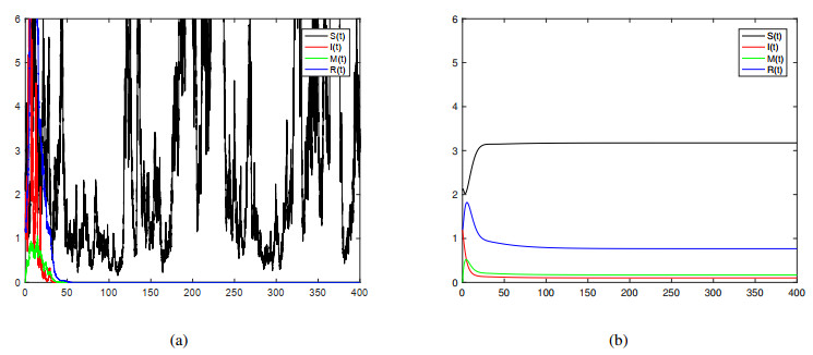
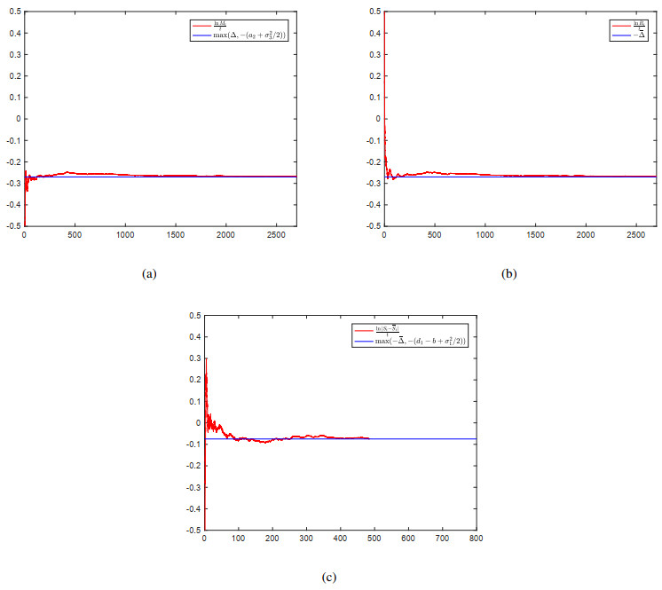
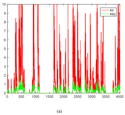
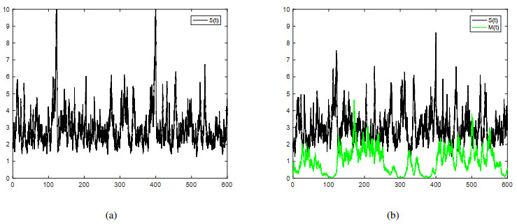
The dynamic behavior of a stochastic epidemic model with information intervention and vertical transmission was the concern of this paper. The threshold to judge the extinction and persistence of the disease is obtained. When $\Delta = \frac{\beta \Lambda}{d_1-b}-(d_1+\gamma+\mu-qb+\frac{1}{2}\sigma_2^2) < 0$, the three classes $I_t$, $M_t$, and $R_t$ appearing in the model go extinct at an exponential rate, and the susceptible class $S_t$ almost surely converges to the solution of the boundary equation exponentially. When $\Delta > 0$, the disease in the model is persistent in the mean. Besides, the existence of invariant probability measure under this condition is proved by constructing proper Lyapunov functions. In addition, the critical case of $\Delta = 0$ is also investigated and it is found that the disease will not be persistent in the mean under some conditions. Several discussions are presented to explain the results and some numerical examples are proposed to verify the obtained results.

A few other issues are worth further studies. This paper analyzes the model with a bilinear incidence rate, while a nonlinear one can be applied to a wider range of circumstances. Therefore, it will be more generic to generalize the model to one with nonlinear incidence. We consider, in this paper, that the stochastic noise is continuously characterized by white noise, and the introduction of more noises such as Markovian switching and L$\rm\acute{e}$vy noise will enable the model to be more realistic. Further research can be conducted on optimizing strategies for some control and prevention measures. We leave these issues for future investigations.

Use of AI tools declaration

The authors declare they have not used Artificial Intelligence (AI) tools in the creation of this article.

Acknowledgments

This research was supported by the Jiangxi Province High level and High skilled Leading Talent Training Project, the Science and Technology projects of Jiangxi Province Education Department (No. GJJ212716) and the National Key R & D Program of China (No. 2023YFC3008902).

Conflict of interest

The authors declare that they have no competing interests.