Threshold dynamics of a stochastic SIRS epidemic model with transfer from infected individuals to susceptible individuals and log-normal Ornstein-Uhlenbeck process

Miaomiao Gao; Yanhui Jiang; Daqing Jiang; Miaomiao Gao; Yanhui Jiang; Daqing Jiang

doi:10.3934/era.2025133

Electronic Research Archive

2025, Volume 33, Issue 5: 3037-3064. doi: 10.3934/era.2025133

Previous Article Next Article

Research article

Threshold dynamics of a stochastic SIRS epidemic model with transfer from infected individuals to susceptible individuals and log-normal Ornstein-Uhlenbeck process

1.
Business college, Qingdao University, Qingdao 266071, China
2.
School of Mathematics and Statistics, Qingdao University, Qingdao 266071, China
3.
College of Science, China University of Petroleum (East China), Qingdao 266580, China

Received: 31 January 2025 Revised: 26 April 2025 Accepted: 28 April 2025 Published: 19 May 2025

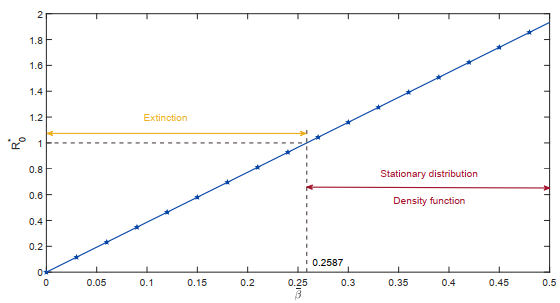
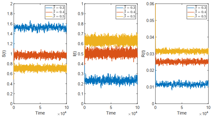
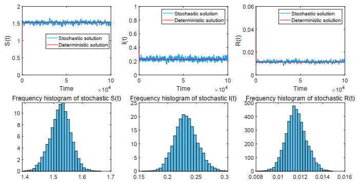
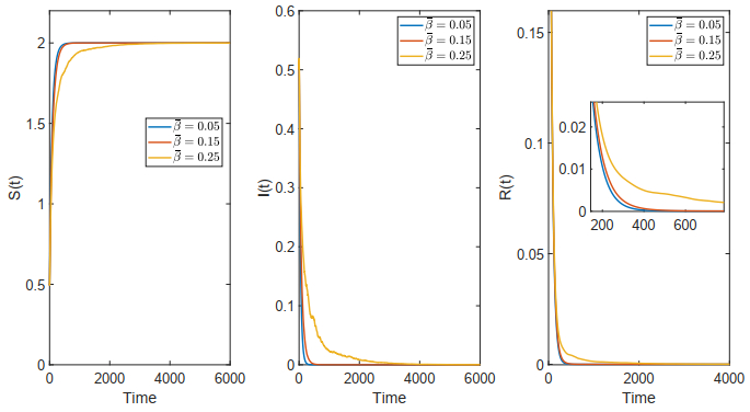
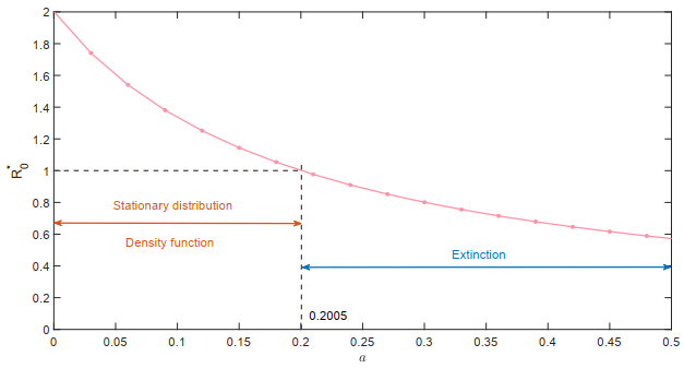
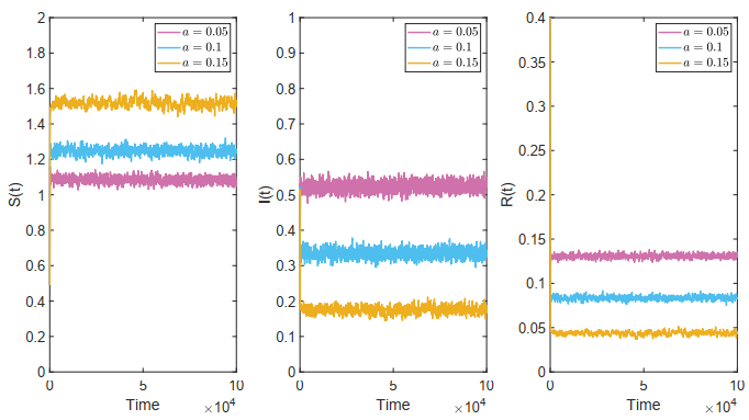
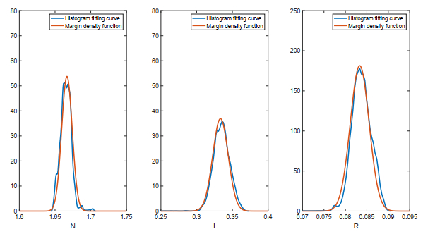
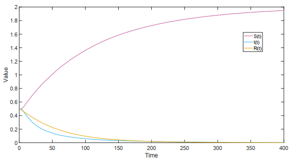
This paper focused on a stochastic susceptible-infected-recovered-susceptible (SIRS) epidemic model with standard incidence and transfer from infected individuals to susceptible individuals. We assumed that the incidence rate satisfied the log-normal Ornstein-Uhlenbeck process. First, by using stochastic Lyapunov analysis method, the sufficient condition for the existence of stationary distribution was obtained. After that, we established the sufficient criteria for the extinction of the infectious disease. It was worth noting that the dynamical behavior of the considered model was governed by a threshold. In addition, we derived the exact expression of probability density function near the positive equilibrium point of the corresponding deterministic system. Finally, some numerical simulations were carried out to confirm theoretical results.
- SIRS model,
- log-normal Ornstein-Uhlenbeck process,
- stationary distribution,
- density function,
- extinction
Citation: Miaomiao Gao, Yanhui Jiang, Daqing Jiang. Threshold dynamics of a stochastic SIRS epidemic model with transfer from infected individuals to susceptible individuals and log-normal Ornstein-Uhlenbeck process[J]. Electronic Research Archive, 2025, 33(5): 3037-3064. doi: 10.3934/era.2025133

Related Papers:

Abstract

This paper focused on a stochastic susceptible-infected-recovered-susceptible (SIRS) epidemic model with standard incidence and transfer from infected individuals to susceptible individuals. We assumed that the incidence rate satisfied the log-normal Ornstein-Uhlenbeck process. First, by using stochastic Lyapunov analysis method, the sufficient condition for the existence of stationary distribution was obtained. After that, we established the sufficient criteria for the extinction of the infectious disease. It was worth noting that the dynamical behavior of the considered model was governed by a threshold. In addition, we derived the exact expression of probability density function near the positive equilibrium point of the corresponding deterministic system. Finally, some numerical simulations were carried out to confirm theoretical results.

References

[1]	W. O. Kermack, A. G. McKendrick, Contributions to the mathematical theory of epidemics-Ⅰ, Proc. Roy. Soc. Lond. Ser. A., 115 (1927), 700–721.
[2]	W. M. Liu, S. A. Levin, Y. Lwasa, Influence of nonlinear incidence rates upon the behavior of SIRS epidemiological models, J. Math. Biol., 23 (1986), 187–204. https://doi.org/10.1007/BF00276956 doi: 10.1007/BF00276956
[3]	Y. Muroya, Y. Enatsu, T. Kuniya, Global stability for a multi-group SIRS epidemic model with varying population sizes, Nonlinear Anal. Real World Appl., 14 (2013), 1693–1704. https://doi.org/10.1016/j.nonrwa.2012.11.005 doi: 10.1016/j.nonrwa.2012.11.005
[4]	M. Sekiguchi, Permanence of a discrete SIRS epidemic model with time delays, Appl. Math. Lett., 23 (2010), 1280–1285. https://doi.org/10.1016/j.aml.2010.06.013 doi: 10.1016/j.aml.2010.06.013
[5]	Y. Z. Bai, X. Q. Mu, Global asymptotic stability of a generalized SIRS epidemic model with transfer from infectious to susceptible, J. Appl. Anal. Comput., 8 (2018), 402–412. https://doi.org/10.11948/2018.402 doi: 10.11948/2018.402
[6]	E. Avila-Vales, A. G. C. Pérez, Dynamics of a reaction-diffusion SIRS model with general incidence rate in a heterogeneous environment, Z. Angew. Math. Phys., 73 (2022). https://doi.org/10.1007/s00033-021-01645-0 doi: 10.1007/s00033-021-01645-0
[7]	J. J. Chen, An SIRS epidemics model, Appl. Math. J. Chin. Univ., 19 (2004), 101–108. https://doi.org/10.1007/s11766-004-0027-8 doi: 10.1007/s11766-004-0027-8
[8]	R. May, Stability and Complexity in Model Ecosystems, Princeton University Press, 2001.
[9]	N. Privault, L. Wang, Stochastic SIR Lévy jump model with heavy-tailed increments, J. Nonlinear Sci., 31 (2021), 15. https://doi.org/10.1007/s00332-020-09670-5 doi: 10.1007/s00332-020-09670-5
[10]	X. B. Zhang, X. D. Wang, H. F. Huo, Extinction and stationary distribution of a stochastic SIRS epidemic model with standard incidence rate and partial immunity, Physica A, 531 (2019), 121548. https://doi.org/10.1016/j.physa.2019.121548 doi: 10.1016/j.physa.2019.121548
[11]	A. Settati, A. Lahrouz, M. E. Jarroudi, M. E. Fatini, K. Wang, On the threshold dynamics of the stochastic SIRS epidemic model using adequate stopping times, Discrete Contin. Dyn. Syst. Ser. B., 25 (2020), 1985–1997. https://doi.org/10.3934/dcdsb.2020012 doi: 10.3934/dcdsb.2020012
[12]	X. Z. Meng, S. N. Zhao, T. Feng, T. H. Zhang, Dynamics of a novel nonlinear stochastic SIS epidemic model with double epidemic hypothesis, J. Math. Anal. Appl., 433 (2015), 227–242. https://doi.org/10.1016/j.jmaa.2015.07.056 doi: 10.1016/j.jmaa.2015.07.056
[13]	A. Tocino, A. M. del Rey, Local stochastic stability of SIRS models without Lyapunov functions, Commun. Nonlinear Sci. Numer. Simul., 103 (2021), 105956. https://doi.org/10.1016/j.cnsns.2021.105956 doi: 10.1016/j.cnsns.2021.105956
[14]	S. P. Rajasekar, M. Pitchaimani, Ergodic stationary distribution and extinction of a stochastic SIRS epidemic model with logistic growth and nonlinear incidence, Appl. Math. Comput., 377 (2020), 125143. https://doi.org/10.1016/j.amc.2020.125143 doi: 10.1016/j.amc.2020.125143
[15]	E. Allen, Environmental variability and mean-reverting processes, Discrete Contin. Dyn. Syst. Ser. B., 21 (2016), 2073–2089. https://doi.org/10.3934/dcdsb.2016037 doi: 10.3934/dcdsb.2016037
[16]	W. M. Wang, Y. L. Cai, Z. Q. Dong, Z. J. Gui, A stochastic differential equation SIS epidemic model incorporating Ornstein-Uhlenbeck process, Physica A, 509 (2018), 921–936. https://doi.org/10.1016/j.physa.2018.06.099 doi: 10.1016/j.physa.2018.06.099
[17]	A. Laaribi, B. Boukanjime, M. E. Khalifi, D. Bouggar, M. E. Fatini, A generalized stochastic SIRS epidemic model incorporating mean-reverting Ornstein-Uhlenbeck process, Physica A, 615 (2023), 128609. https://doi.org/10.1016/j.physa.2023.128609 doi: 10.1016/j.physa.2023.128609
[18]	Z. C. Wu, D. Q. Jiang, Dynamics and density function of a stochastic SICA model of a standard incidence rate with Ornstein-Uhlenbeck process, Qual. Theory Dyn. Syst., 23 (2024), 219. https://doi.org/10.1007/s12346-024-01073-1 doi: 10.1007/s12346-024-01073-1
[19]	P. Saha, K. K. Pal, U. Ghosh, P. K. Tiwari, Dynamic analysis of deterministic and stochastic SEIR models incorporating the Ornstein-Uhlenbeck process, Chaos, 35 (2025), 023165. https://doi.org/10.1063/5.0243656 doi: 10.1063/5.0243656
[20]	Y. Zhao, S. L. Yuan, J. L. Ma, Survival and stationary distribution analysis of a stochastic competitive model of three species in a polluted environment, Bull. Math. Biol., 77 (2015), 1285–1326. https://doi.org/10.1007/s11538-015-0086-4 doi: 10.1007/s11538-015-0086-4
[21]	M. M. Gao, D. Q. Jiang, J. Y. Ding, Dynamical behavior of a nutrient-plankton model with Ornstein-Uhlenbeck process and nutrient recycling, Chaos, Solitons Fractals, 174 (2023), 113763. https://doi.org/10.1016/j.chaos.2023.113763 doi: 10.1016/j.chaos.2023.113763
[22]	N. T. Dieu, Asymptotic properties of a stochastic SIR epidemic model with Beddington-DeAngelis incidence rate, J. Dyn. Differ. Equations, 30 (2018), 93–106. https://doi.org/10.1007/s10884-016-9532-8 doi: 10.1007/s10884-016-9532-8
[23]	S. P. Meyn, R. L. Tweedie, Stability of Markovian processes Ⅲ: Foster-Lyapunov criteria for continuous-time processes, Adv. Appl. Probab., 25 (1993), 518–548. https://doi.org/10.2307/1427522 doi: 10.2307/1427522
[24]	N. H. Du, D. H. Nguyen, G. G. Yin, Conditions for permanence and ergodicity of certain stochastic predator-prey models, J. Appl. Probab., 53 (2016), 187–202. https://doi.org/10.1017/jpr.2015.18 doi: 10.1017/jpr.2015.18
[25]	X. Mao, C. Yuan, Stochastic Differential Equations with Markovian Switching, Imperial College Press, London, 2006. https://doi.org/10.1142/p473
[26]	Z. E. Ma, Y. C. Zhou, C. Z. Li, Qualitative and Stability Methods for Ordinary Differential Equations, Science Press, Beijing, 2015.
[27]	D. J. Higham, An algorithmic introduction to numerical simulation of stochastic differential equations, SIAM Rev., 43 (2001), 525–546. https://doi.org/10.1137/S0036144500378302 doi: 10.1137/S0036144500378302

Reader Comments

Your name:*

Email:*
© 2025 the Author(s), licensee AIMS Press. This is an open access article distributed under the terms of the Creative Commons Attribution License (http://creativecommons.org/licenses/by/4.0)