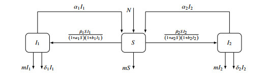
The host population in epidemiology may actually be at risk of more than two infectious diseases with stochastic complicated interaction, e.g., HIV and HBV. In this paper, we propose a class of stochastic epidemic model that applies the double epidemic hypothesis and Crowley-Martin incidence rate in order to explore how stochastic disturbances affect the spread of diseases. While disregarding stochastic disturbances, we examine the dynamic features of the system in which the local stability of equilibria are totally determined by the basic reproduction numbers. We focus particularly on the threshold dynamics of the corresponding stochastic system, and we obtain the extinction and permanency conditions for a pair of infectious diseases. We find that the threshold dynamics of the deterministic and stochastic systems vary significantly: (ⅰ) disease outbreaks can be controlled by appropriate stochastic disturbances; (ⅱ) diseases die out when the intensity of environmental perturbations is higher. The effects of certain important parameters on deterministic and stochastic disease transmission were obtained through numerical simulations. Our observations indicate that controlling epidemics should improve the effectiveness of prevention measures for susceptible individuals while improving the effectiveness of treatment for infected individuals.
Citation: Wenxuan Li, Suli Liu. Dynamic analysis of a stochastic epidemic model incorporating the double epidemic hypothesis and Crowley-Martin incidence term[J]. Electronic Research Archive, 2023, 31(10): 6134-6159. doi: 10.3934/era.2023312
The host population in epidemiology may actually be at risk of more than two infectious diseases with stochastic complicated interaction, e.g., HIV and HBV. In this paper, we propose a class of stochastic epidemic model that applies the double epidemic hypothesis and Crowley-Martin incidence rate in order to explore how stochastic disturbances affect the spread of diseases. While disregarding stochastic disturbances, we examine the dynamic features of the system in which the local stability of equilibria are totally determined by the basic reproduction numbers. We focus particularly on the threshold dynamics of the corresponding stochastic system, and we obtain the extinction and permanency conditions for a pair of infectious diseases. We find that the threshold dynamics of the deterministic and stochastic systems vary significantly: (ⅰ) disease outbreaks can be controlled by appropriate stochastic disturbances; (ⅱ) diseases die out when the intensity of environmental perturbations is higher. The effects of certain important parameters on deterministic and stochastic disease transmission were obtained through numerical simulations. Our observations indicate that controlling epidemics should improve the effectiveness of prevention measures for susceptible individuals while improving the effectiveness of treatment for infected individuals.

| [1] |
Y. Xu, X. Sun, H. Hu, Extinction and stationary distribution of a stochastic SIQR epidemic model with demographics and non-monotone incidence rate on scale-free networks, J. Appl. Math. Comput., 68 (2021), 3367–3395. https://doi.org/10.1007/s12190-021-01645-3 doi: 10.1007/s12190-021-01645-3

|
| [2] |
R. Zhao, Q. Liu, M. Sun, Dynamical behavior of a stochastic SIQS epidemic model on scale-free networks, J. Appl. Math. Comput., 68 (2021), 813–838. https://doi.org/10.1007/s12190-021-01550-9 doi: 10.1007/s12190-021-01550-9
|
| [3] |
S. Bera, S. Khajanchi, T. K. Roy, Stability analysis of fuzzy HTLV-Ⅰ infection model: a dynamic approach, J. Appl. Math. Comput., 69 (2022), 171–199. https://doi.org/10.1007/s12190-022-01741-y doi: 10.1007/s12190-022-01741-y
|
| [4] |
H. Guo, M. Li, Z. Shuai, Global dynamics of a general class of multistage models for infectious diseases, SIAM J. Appl. Math., 72 (2012), 261–279. https://doi.org/10.1137/110827028 doi: 10.1137/110827028
|
| [5] |
Y. Cai, S. Zhao, Y. Niu, Z. Peng, K. Wang, D. He, et al., Modelling the effects of the contaminated environments on tuberculosis in Jiangsu, China, J. Theor. Biol., 508 (2021), 110453. https://doi.org/10.1016/j.jtbi.2020.110453 doi: 10.1016/j.jtbi.2020.110453
|
| [6] |
X. Guan, F. Yang, W. Wang, Global stability of an influenza A model with vaccination, Appl. Math. Lett., 134 (2022), 0893–9659. https://doi.org/10.1016/j.aml.2022.108322 doi: 10.1016/j.aml.2022.108322
|
| [7] |
Y. Nie, X. Zhong, T. Lin, W. Wang, Pathogen diversity in meta-population networks, Chaos Solitons Fractals, 166 (2023), 112909. https://doi.org/10.1016/j.chaos.2022.112909 doi: 10.1016/j.chaos.2022.112909
|
| [8] |
Y. Nie, W. Li, L. Pan, T. Lin, W. Wang, Markovian approach to tackle competing pathogens in simplicial complex, Appl. Math. Comput., 417 (2022), 126773. https://doi.org/10.1016/j.amc.2021.126773 doi: 10.1016/j.amc.2021.126773
|
| [9] |
Y. Nie, X. Zhong, T. Lin, W. Wang, Homophily in competing behavior spreading among the heterogeneous population with higher-order interactions, Appl. Math. Comput., 432 (2022), 127380. https://doi.org/10.1016/j.amc.2022.127380 doi: 10.1016/j.amc.2022.127380
|
| [10] |
W. O. Kermack, A. G. McKendrick, A contribution to the mathematical theory of epidemics, Proc. R. Soc. London, Ser. A, 115 (1927), 700–721. https://doi.org/10.1098/rspa.1927.0118 doi: 10.1098/rspa.1927.0118
|
| [11] |
X. Zhang, M. Liu, Dynamical analysis of a stochastic delayed SIR epidemic model with vertical transmission and vaccination, Adv. Contin. Discrete Modelss, 1 (2022). https://doi.org/10.1186/s13662-022-03707-7 doi: 10.1186/s13662-022-03707-7
|
| [12] |
Q. Li, Z. Lin, A diffusive SIS epidemic model in a heterogeneous and periodically evolvingenvironment, Math. Biosci. Eng., 16 (2019), 3094–3110. https://doi.org/10.3934/mbe.2019153 doi: 10.3934/mbe.2019153
|
| [13] |
Q. Pan, J. Huang, H. Wang, An SIRS model with nonmonotone incidence and saturated treatment in a changing environment, J. Math. Biol., 85 (2022). https://doi.org/10.1007/s00285-022-01787-3 doi: 10.1007/s00285-022-01787-3
|
| [14] |
L. Yang, Y. Li, Periodic traveling waves in a time periodic SEIR model with nonlocal dispersal and delay, Discrete Contin. Dyn. Syst. B, 28 (2023), 5087–5104. https://doi.org/10.3934/dcdsb.2023056 doi: 10.3934/dcdsb.2023056
|
| [15] |
A. Franceschetti, A. Pugliese, D. Breda, Multiple endemic states in age-structured SIR epidemic models, Math. Biosci. Eng., 9 (2012), 577–599. https://doi.org/10.3934/mbe.2012.9.577 doi: 10.3934/mbe.2012.9.577
|
| [16] |
C. Zhang, J. Gao, H. Sun, J. Wang, Dynamics of a reaction diffusion SVIR model in a spatial heterogeneous environment, Physica A, 533 (2019), 122049. https://doi.org/10.1016/j.physa.2019.122049 doi: 10.1016/j.physa.2019.122049
|
| [17] |
G. Liu, S. Liu, M. Y. Li, A discrete state-structured model on networks withtwo transmission modes: Global dynamics analysis, Discrete Contin. Dyn. Syst. B, 28 (2023), 3414–3427. https://doi.org/10.3934/dcdsb.2022224 doi: 10.3934/dcdsb.2022224
|
| [18] |
S. Liu, G. Liu, H. Li, Discrete state-structured epidemic models with distributed delays, Int. J. Biomath., 15 (2022), 2250040. https://doi.org/10.1142/S1793524522500401 doi: 10.1142/S1793524522500401
|
| [19] |
S. Liu, M. Y. Li, Epidemic models with discrete state structures, Physica D, 422 (2021), 132903. https://doi.org/10.1016/j.physd.2023.133884 doi: 10.1016/j.physd.2023.133884
|
| [20] |
L. Weldemhret, Epidemiology and challenges of HBV/HIV co-infection amongst HIV-infected patients in endemic areas, HIV/AIDS-Res. Palliative Care, 13 (2021), 485–490. https://doi.org/10.2147/hiv.s273649 doi: 10.2147/hiv.s273649
|
| [21] |
J. S. Casalegno, M. Ottmann, M. B. Duchamp, V. Escuret, G. Billaud, E. Frobert, et al., Rhinoviruses delayed the circulation of the pandemic influenza A (H1N1) 2009 virus in France, Clin. Microbiol. Infect., 16 (2010), 326–329. https://doi.org/10.1111/j.1469-0691.2010.03167.x doi: 10.1111/j.1469-0691.2010.03167.x
|
| [22] |
Y. Liu, A. Feng, S. Zhao, W. Wang, D. He, Large-scale synchronized replacement of Alpha (B.1.1.7) variant by the Delta (B.1.617.2) variant of SARS-COV-2 in the COVID-19 pandemic, Math. Biosci. Eng., 19 (2022), 3591–3596. https://doi.org/10.3934/mbe.2022165 doi: 10.3934/mbe.2022165
|
| [23] |
A. Miao, X. Wang, T. Zhang, W. Wang, B. S. A. Pradeep, Dynamical analysis of a stochastic SIS epidemic model with nonlinear incidence rate and double epidemic hypothesis, Adv. Differ. Equations, 2017 (2017). https://doi.org/10.1186/s13662-017-1289-9 doi: 10.1186/s13662-017-1289-9
|
| [24] |
Q. Liu, D. Jiang, T. Hayat, A. Alsaedi, Threshold behavior in a stochastic delayed SIS epidemic model with vaccination and double diseases, J. Franklin Inst., 356 (2019), 7466–7485. https://doi.org/10.1016/j.jfranklin.2018.11.055 doi: 10.1016/j.jfranklin.2018.11.055
|
| [25] |
J. Zhang, Y. Chu, W. Du, Y. Chang, X. An, Stability and hopf bifurcation in a delayed SIS epidemic model with double epidemic hypothesis, Int. J. Nonlinear Sci., 19 (2018), 561–571. https://doi.org/10.1515/ijnsns-2016-0122 doi: 10.1515/ijnsns-2016-0122
|
| [26] |
W. O. Kermack, A. G. McKendrick, Contributions to the mathematical theory of epidemics—Ⅰ, Bull. Math. Biol., 53 (1991), 33–55. https://doi.org/10.1007/bf02464423 doi: 10.1007/bf02464423
|
| [27] |
Z. Hu, S. Liu, H. Wang, Backward bifurcation of an epidemic model with standard incidence rate and treatment rate, Nonlinear Anal. Real World Appl., 9 (2008), 2302–2312. https://doi.org/10.1016/j.nonrwa.2007.08.009 doi: 10.1016/j.nonrwa.2007.08.009
|
| [28] |
Y. Yang, D. Xiao, Influence of latent period and nonlinear incidence rate on the dynamics of SIRS epidemiological models, Discrete Contin. Dyn. Syst. B, 13 (2010), 195–211. https://doi.org/10.3934/dcdsb.2010.13.195 doi: 10.3934/dcdsb.2010.13.195
|
| [29] |
Y. Cai, J. Li, Y. Kang, K. Wang, W. Wang, The fluctuation impact of human mobility on the influenza transmission, J. Franklin Inst., 357 (2020), 8899–8924. https://doi.org/10.1016/j.jfranklin.2020.07.002 doi: 10.1016/j.jfranklin.2020.07.002
|
| [30] |
P. H. Crowley, E. K. Martin, Functional responses and interference within and between year classes of a dragonfly population, J. N. Am. Benthological Soc., 8 (1989), 211–221. https://doi.org/10.2307/1467324 doi: 10.2307/1467324
|
| [31] |
J. P. Tripathi, S. Tyagi, S. Abbas, Global analysis of a delayed density dependent predator–prey model with Crowley–Martin functional response, Commun. Nonlinear Sci. Numer. Simul., 30 (2016), 45–69. https://doi.org/10.1016/j.cnsns.2015.06.008 doi: 10.1016/j.cnsns.2015.06.008
|
| [32] |
H. Huo, F. Zhang, H. Xiang, Spatiotemporal dynamics for impulsive eco-epidemiological model with Crowley-Martin type functional response, Math. Biosci. Eng., 19 (2022), 12180–12211. https://doi.org/10.3934/mbe.2022567 doi: 10.3934/mbe.2022567
|
| [33] |
A. Mohsen, H. Husseiny, K. Hattaf, The awareness effect of the dynamical behavior of SIS epidemic model with Crowley-Martin incidence rate and holling type Ⅲ treatment function, Int. J. Nonlinear Anal. Appl., 12 (2021), 1083–1097. https://doi.org/10.22075/ijnaa.2021.5177 doi: 10.22075/ijnaa.2021.5177
|
| [34] |
A. Kumar, Dynamic behavior of an SIR epidemic model along with time delay; Crowley–Martin type incidence rate and holling type Ⅱ treatment rate, Int. J. Nonlinear Sci., 20 (2019), 757–771. https://doi.org/10.1515/ijnsns-2018-0208 doi: 10.1515/ijnsns-2018-0208
|
| [35] |
Y. Liu, C. Wu, Global dynamics for an HIV infection model with Crowley-Martin functional response and two distributed delays, J. Syst. Sci. Complexity, 31 (2017), 385–395. https://doi.org/10.1007/s11424-017-6038-3 doi: 10.1007/s11424-017-6038-3
|
| [36] |
W. Wang, Modeling adaptive behavior in influenza transmission, Math. Modell. Nat. Phenom., 7 (2012), 253–262. https://doi.org/10.1051/mmnp/20127315 doi: 10.1051/mmnp/20127315
|
| [37] |
F. Wang, Z. Liu, Dynamical behavior of a stochastic SIQS model via isolation with regime-switching, J. Appl. Math. Comput., 69 (2022), 2217–2237. https://doi.org/10.1007/s12190-022-01831-x doi: 10.1007/s12190-022-01831-x
|
| [38] |
M. Mehdaoui, A. L. Alaoui, M. Tilioua, Dynamical analysis of a stochastic non-autonomous SVIR model with multiple stages of vaccination, J. Appl. Math. Comput., 69 (2022), 2217–2206. https://doi.org/10.1007/s12190-022-01828-6 doi: 10.1007/s12190-022-01828-6
|
| [39] |
S. He, S. Tang, L. Rong, A discrete stochastic model of the COVID-19 outbreak: Forecast and control, Math. Biosci. Eng., 17 (2020), 2792–2804. https://doi.org/10.3934/mbe.2020153 doi: 10.3934/mbe.2020153
|
| [40] |
A. Gray, X. Mao, D. Jiang, Y. Zhao, The threshold of a stochastic SIRS epidemic model in a population with varying size, Discrete Contin. Dyn. Syst. - Ser. B, 20 (2015), 1277–1295. https://doi.org/10.3934/dcdsb.2015.20.1277 doi: 10.3934/dcdsb.2015.20.1277
|
| [41] |
M. T. Anche, M. D. Jong, P. Bijma, On the definition and utilization of heritable variation among hosts in reproduction ratio R0 for infectious diseases, Heredity, 113 (2014), 364–374. https://doi.org/10.1038/hdy.2014.38 doi: 10.1038/hdy.2014.38
|
| [42] |
P. van den Driessche, J. Watmough, Reproduction numbers and sub-threshold endemic equilibria for compartmental models of disease transmission, Math. Biosci., 180 (2002), 29–48. https://doi.org/10.1016/s0025-5564(02)00108-6 doi: 10.1016/s0025-5564(02)00108-6
|
| [43] | R. Z. Khas'miniskii, Stochastic Stability of Differential Equations, Springer Berlin Heidelberg, 1980. https://doi.org/10.1007/978-94-009-9121-7 |
| [44] |
Q. Liu, D. Jiang, T. Hayat, A. Alsaedi, B. Ahmad, A stochastic SIRS epidemic model with logistic growth and general nonlinear incidence rate, Phys. A, 551 (2020), 124152. https://doi.org/10.1016/j.physa.2020.124152 doi: 10.1016/j.physa.2020.124152
|
| [45] | X. Mao, Stochastic Differential Equations and Applications, Horwood, Chichester, 2008. https://doi.org/10.1533/9780857099402 |
| [46] |
P. E. Kloeden, E. Platen, Higher-order implicit strong numerical schemes for stochastic differential equations, J. Stat. Phys., 66 (1992), 283–314. https://doi.org/10.1007/bf01060070 doi: 10.1007/bf01060070
|
| [47] |
X. Meng, S. Zhao, T. Feng, T. Zhang, Dynamics of a novel nonlinear stochastic SIS epidemic model with double epidemic hypothesis, J. Math. Anal. Appl., 433 (2016), 227–242. https://doi.org/10.1016/j.jmaa.2015.07.056 doi: 10.1016/j.jmaa.2015.07.056
|
Figures(7) / Tables(1)
Wenxuan Li, Suli Liu. Dynamic analysis of a stochastic epidemic model incorporating the double epidemic hypothesis and Crowley-Martin incidence term[J]. Electronic Research Archive, 2023, 31(10): 6134-6159. doi: 10.3934/era.2023312


 DownLoad: