Transition characteristics of the dynamic behavior of a vehicle wheel-rail vibro-impact system

Yang Jin; Wanxiang Li; Hongbing Zhang; Yang Jin; Wanxiang Li; Hongbing Zhang

doi:10.3934/era.2023357

Electronic Research Archive

2023, Volume 31, Issue 11: 7040-7060. doi: 10.3934/era.2023357

Previous Article Next Article

Theory article Special Issues

Transition characteristics of the dynamic behavior of a vehicle wheel-rail vibro-impact system

School of Mechanical and Electrical Engineering, Lanzhou Jiaotong University, Lanzhou 730070, China

Received: 15 August 2023 Revised: 19 October 2023 Accepted: 25 October 2023 Published: 02 November 2023

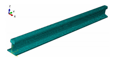
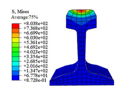
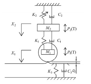
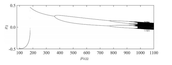
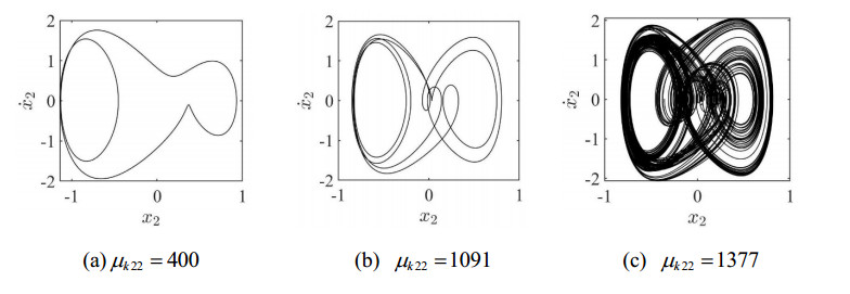
A two-degree-of-freedom vehicle wheel-rail impact vibration system model is developed, and the equivalent impact stiffness and damping of the rail are fitted applying ABAQUS, taking into account the high and low irregularity generated by the welded joints of the rail. A wheel-rail periodic interface with fixed impact was selected as the Poincaré map, and the fourth-order Runge-Kutta numerical method with variable step size was used to solve the system response. The dynamic characteristics of the system are investigated using a combination of the Bifurcation diagram, Phase plane diagram, the Poincaré map, the Time-domain diagram and the Frequency-domain diagram. It is verified that the vehicle wheel-rail impact vibration system has Hopf bifurcation, Neimark-Sacker bifurcation, Period-doubling bifurcation and Boundary crisis, and there are rich and complex nonlinear dynamic behavior changes. The research on the bifurcation and chaos characteristics of vehicle wheel-rail impact vibration systems can provide a reference for improving the stability of vehicle operation in engineering practice as well as the prediction and control of chaos in vehicle vibration reduction design.

Keywords:

Citation: Yang Jin, Wanxiang Li, Hongbing Zhang. Transition characteristics of the dynamic behavior of a vehicle wheel-rail vibro-impact system[J]. Electronic Research Archive, 2023, 31(11): 7040-7060. doi: 10.3934/era.2023357

Related Papers:

[1]	María Ángeles García-Ferrero, Angkana Rüland . Strong unique continuation for the higher order fractional Laplacian. Mathematics in Engineering, 2019, 1(4): 715-774. doi: 10.3934/mine.2019.4.715
[2]	Chiara Gavioli, Pavel Krejčí . Deformable porous media with degenerate hysteresis in gravity field. Mathematics in Engineering, 2025, 7(1): 35-60. doi: 10.3934/mine.2025003
[3]	Fernando Farroni, Gioconda Moscariello, Gabriella Zecca . Lewy-Stampacchia inequality for noncoercive parabolic obstacle problems. Mathematics in Engineering, 2023, 5(4): 1-23. doi: 10.3934/mine.2023071
[4]	Federico Cluni, Vittorio Gusella, Dimitri Mugnai, Edoardo Proietti Lippi, Patrizia Pucci . A mixed operator approach to peridynamics. Mathematics in Engineering, 2023, 5(5): 1-22. doi: 10.3934/mine.2023082
[5]	Francesco Maddalena, Danilo Percivale, Franco Tomarelli . Signorini problem as a variational limit of obstacle problems in nonlinear elasticity. Mathematics in Engineering, 2024, 6(2): 261-304. doi: 10.3934/mine.2024012
[6]	Xavier Fernández-Real, Alessio Figalli . On the obstacle problem for the 1D wave equation. Mathematics in Engineering, 2020, 2(4): 584-597. doi: 10.3934/mine.2020026
[7]	Patrizia Pucci, Letizia Temperini . On the concentration–compactness principle for Folland–Stein spaces and for fractional horizontal Sobolev spaces. Mathematics in Engineering, 2023, 5(1): 1-21. doi: 10.3934/mine.2023007
[8]	Petteri Harjulehto, Peter Hästö, Jonne Juusti . Bloch estimates in non-doubling generalized Orlicz spaces. Mathematics in Engineering, 2023, 5(3): 1-21. doi: 10.3934/mine.2023052
[9]	Luca Spolaor, Bozhidar Velichkov . On the logarithmic epiperimetric inequality for the obstacle problem. Mathematics in Engineering, 2021, 3(1): 1-42. doi: 10.3934/mine.2021004
[10]	Boubacar Fall, Filippo Santambrogio, Diaraf Seck . Shape derivative for obstacles in crowd motion. Mathematics in Engineering, 2022, 4(2): 1-16. doi: 10.3934/mine.2022012

Abstract

1. Introduction

Let $n$ and $k$ be two positive integers. Denote by $p\left(n, k\right)$ the number of partitions of the positive number $n$ on exactly $k$ parts. Then the partition class $k$ is the sequence $p\left(1, k\right), p\left(2, k\right), \dots, p\left(n, k\right), \dots$ We already know, see ^[1], all these values can be divided into the highest $d_0 = LCM\left(1, 2, \dots, k\right)$ sub sequences, each of which is calculated by the same polynomial.

Choose a sequence of $k$ natural numbers such that: the first member is arbitrary, and the rest form an arithmetic progression with a difference $d = m\cdot d_0, \enspace m \in \mathbb{N}$ , starting from the chosen first member. For example:

$\begin{equation} x_1 = j, \enspace x_2 = j+d, \enspace \dots, \enspace x_k = j+\left(k-1\right)\cdot d, \quad j\in \mathbb{N}. \end{equation}$

(1.1)

The corresponding number of partitions of the class $k$ for the elements of the previous arithmetic progression's values is:

$\begin{equation} p\left(x_1, k\right), \enspace p\left(x_2, k\right), \enspace \dots \enspace, \enspace p\left(x_k, k\right). \end{equation}$

(1.2)

If the values, which are calculated using the same polynomial, multiplied by the corresponding binomial coefficients, form the alternate sum, we notice that the sum always has a value which is independent of $x_1$ , no matter how we form the sequence (1.1).

For the partition function of classes we already know the following results, see ^[1,2] for some details:

ⅰ) The values of the partition function of classes is calculated with one quasi polynomial.

ⅱ) For each class $k$ the quasi polynomial consists of at most $LCM\left(1, 2, \dots, k\right)$ different polynomials, each of them consists of a strictly positive and an alternating part.

ⅲ) All polynomials within one quasi polynomial $p\left(n, k\right)$ are of degree $k-1$ .

ⅳ) All the coefficients with the highest degrees down to $\left[\frac{k}{2}\right]$ are equal for all polynomials (all of strictly positive) and all polynomials differ only in lower coefficients (alternating part).

ⅴ) The form of any polynomial $p\left(n, k\right)$ is:

$\begin{equation} p\left(n, k\right) = a_1n^{k-1}+a_2n^{k-2}+\dots+a_k, \end{equation}$

(1.3)

where the coefficients $a_1, a_2, \dots, a_k$ are calculated in the general form.

Let us forget for a moment that the coefficients $a_1, a_2, \dots$ are known in general form. Knowing that all values for partitions class of the sequence (1.1) are obtained by one polynomial $p\left(n, k\right)$ , it is possible to determine all unknown coefficients in a completely different way from that given in papers ^[1,2]. To determine $k$ unknowns, a $k$ equation is required. For this purpose, it is sufficient to know all the values of the sequence (1.2). To this end, we must form the system (1.4) and solve it. (For $k = 10$ , see ^[3]).

$\begin{equation} \begin{split} & a_1\cdot x_1^{k-1}+a_2\cdot x_1^{k-2}+\dots+a_k = p\left(x_1, k\right)\\ & a_1\cdot x_2^{k-1}+a_2\cdot x_2^{k-2}+\dots+a_k = p\left(x_2, k\right)\\ & \dots \quad \dots \quad \dots\\ & a_1\cdot x_k^{k-1}+a_2\cdot x_k^{k-2}+\dots+a_k = p\left(x_k, k\right) \end{split} \end{equation}$

(1.4)

The system (1.4) can be solved by Cramer's Rule. For further analysis, we need to find the following determinants. We will start with the known Vandermonde determinant, see ^[4].

$\begin{equation} \Delta_m = \begin{vmatrix} x_{1}^{m-1} & x_{1}^{m-2} & \dots & 1 \\ x_{2}^{m-1} & x_{2}^{m-2} & \dots & 1 \\ \dots & \dots & \dots \\ x_m^{m-1} & x_m^{m-2} & \dots & 1 \\ \end{vmatrix} = \prod\limits_{1 \le i \lt j \le m}\left(x_i-x_j\right), \enspace m \gt 1. \end{equation}$

(1.5)

When we remove the first column and an arbitrary row from the previous determinant we obtain the Vandermonde determinant of one order less. The following results are known, see ^[4] and are needed for further exposure. If we remove the second column and an arbitrary $a$ -th row from the determinant (1.5) we get

$\begin{equation} \begin{vmatrix} x_1^{m-1} & x_1^{m-3} & \dots & x_1 & 1 \\ \dots & \dots & \dots & \dots & \dots \\ x_{a-1}^{m-1} & x_{a-1}^{m-3} & \dots & x_{a-1} & 1 \\ x_{a+1}^{m-1} & x_{a+1}^{m-3} & \dots & x_{a+1} & 1 \\ \dots & \dots & \dots & \dots & \dots \\ x_m^{m-1} & x_m^{m-3} & \dots & x_m & 1 \\ \end{vmatrix} = \left(\sum\limits_{0 \le i\le m}^{i\ne a}x_i\right)\cdot \prod\limits_{0 \le i \lt j \le m}^{i, j\ne a}\left(x_i-x_j\right) \end{equation}$

(1.6)

If we remove the third column and an arbitrary $a$ -th row from the determinant (1.5) we get

$\begin{equation} \begin{vmatrix} x_1^{m-1} & x_1^{m-2} & x_1^{m-4} &\dots & x_1 & 1 \\ \dots & \dots & \dots & \dots & \dots & \dots \\ x_{a-1}^{m-1} & x_{a-1}^{m-2} & x_{a-1}^{m-4} \dots & x_{a-1} & 1 \\ x_{a+1}^{m-1} & x_{a+1}^{m-2} & x_{a+1}^{m-4} \dots & x_{a+1} & 1 \\ \dots & \dots & \dots & \dots & \dots & \dots \\ x_m^{m-1} & x_m^{m-2} & x_m^{m-4} & \dots & x_m & 1 \\ \end{vmatrix} = \sum\limits_{1 \le i \lt j \le m}^{i, j \ne a}x_i \cdot x_j \prod\limits_{0 \le i \lt j\le m}^{i, j \ne a}\left(x_i-x_j\right) \end{equation}$

(1.7)

Generaly, if we remove the $b$ -th column and an arbitrary $a$ -th row from the determinant (1.5) we get

$\begin{multline*} \Delta_{m}^{\left(a, b\right)} = \begin{vmatrix} x_1^{m-1} & x_1^{m-2} & \dots & x_1^{b+1} & x_1^{b-1} & \dots& x_1 & 1 \\ \dots & \dots & \dots & \dots & \dots & \dots & \dots\\ x_{a-1}^{m-1} & x_{a-1}^{m-2} & \dots & x_{a-1}^{b+1} & x_{a-1}^{b-1} & \dots & x_{a-1} & 1 \\ x_{a+1}^{m-1} & x_{a+1}^{m-2} & \dots & x_{a+1}^{b+1} & x_{a+1}^{b-1} & \dots & x_{a+1} & 1 \\ \dots & \dots & \dots & \dots & \dots & \dots & \dots\\ x_m^{m-1} & x_m^{m-2} & \dots & x_m^{b+1} & x_m^{b-1} & \dots & x_m & 1 \\ \end{vmatrix} = \left(\sum\limits_{1 \le t_1 \lt t_2 \dots \lt t_{b-1} \le m}^{t_1, \dots, t_{b-1} \ne a}x_{t_1}x_{t_2} \dots x_{t_{b-1}}\right) \prod\limits_{0\le i \lt j\le m}^{i, j\ne a}\left(x_i-x_j\right). \end{multline*}$

The label $\Delta_{m}^{\left(a, b\right)}$ means that from $\Delta_m$ remove the $a$ -th row and $b$ -th column from the set of variables $x_a$ .

2. Invariants of the partitions classes

2.1. The first partition invariant of classes

Theorem 1. Let $m, j$ and $k$ be three positive integers and

$I_1\left(k, j, d\right) = \sum\limits_{i = 0}^{k-1}\left(-1\right)^i \binom{k-1}{i}p\left(j+i\cdot d, k\right),$

where $d = m\cdot LCM\left(1, 2, 3, \dots, k\right)$ . Then $I_1\left(k, j, d\right) = \left(-1\right)^{k-1}\frac{d^{k-1}}{k!}$ and is independent of $j$ . ( $I_1\left(k, j, d\right)$ is the first partition invariant which exists in all classes.)

Proof. Among the values of the class $k$ we choose the ones corresponding to the sequence (1.1), and they are given with the sequence (1.2). According to ^[2], all the elements in (1.2) can be calculated using the same polynomial $p\left(n, k\right)$ with degree $k-1$ . Elements of the following sequence:

$q, q+d, \dots, q+\left(k-1\right)\cdot d, \quad q \ne j,$

are calculated with not necessarily the same polynomial as the previous one. Let the polynomial $p\left(n, k\right)$ have the form as in (1.3). To determine the coefficients $a_1, a_2, \dots, a_k$ it suffices to know the $k$ values: $p\left(x_1, k\right), p\left(x_2, k\right), \dots, p\left(x_k, k\right)$ where $x_1 = j, \enspace x_2 = j+d, \dots, \enspace x_k = j+\left(k-1\right)d\enspace$ are different numbers. Since $\Delta_k \ne 0$ , system (1.4) always has a unique solution, because all the elements of the set $\left\{x_1, x_2, \dots, x_k\right\}$ are different from one another. According to Cramer's Rule, to determine the coefficient of the highest degree of the polynomial (1.3), which calculates the value of the number of partitions of class $k$ , we have the following formula:

$\begin{equation} a_1 = \frac{p\left(x_1, k\right)\Delta_{k}^{\left(1, 1\right)}-p\left(x_2, k\right)\Delta_{k}^{\left(2, 1\right)}+\dots+\left(-1\right)^{k-1}p\left(x_k, k\right)\Delta_{k}^{\left(k, 1\right)}} {\Delta_k} \end{equation}$

(2.1)

Determinants $\Delta_{k}^{\left(a, 1\right)}, \left(1 \le a \le k\right)$ are also Vandermonde and their values are equal to $\Delta_{k-1}$ . Let $\left\{x_i\right\}_{1\le i \le k}$ satisfy (1.1) then for $1\le a \le k$ it holds that

$\begin{multline*} \Delta_{k}^{\left(a, 1\right)} = \Delta_{k-1} = \frac{\Delta_k}{\prod\limits_{i = 1}^{a-1}\left(x_i-x_a\right)\prod\limits_{i = a+1}^{k}\left(x_a-x_i\right)}\\ = \frac{\Delta_k}{\left(-1\right)^{a-1}\left(a-1\right)!d^{a-1}\cdot \left(-1\right)^{k-a}\left(k-a\right)!d^{k-a}} \\ = \frac{\left(-1\right)^{k-1}\Delta_k}{\left(a-1\right)!\left(k-a\right)!d^{k-1}}. \end{multline*}$

Replacing in (2.1), after shortening with $\Delta_k$ we have

$\begin{multline*} \quad \quad \quad \quad \quad \quad \quad a_1 = \left(-1\right)^{k-1}\left( \frac{p\left(x_1, k\right)}{0!\left(k-1\right)!d^{k-1}}-\frac{p\left(x_2, k\right)}{1!\left(k-2\right)!d^{k-1}}+\dots \right. \left. +\left(-1\right)^{k-1}\frac{p\left(x_k, k\right)}{\left(k-1\right)!0!d^{k-1}}\right). \end{multline*}$

The coefficient $a_1$ is already defined in ^[2] where it is shown that $a_1 = \frac{1}{k!\left(k-1\right)!}$ . Substituting into the previous equality and multiplying by $\left(-1\right)^{k-1}$ , we obtain

$\begin{equation*} \quad \quad \quad \quad \frac{\left(-1\right)^{k-1}}{k!\left(k-1\right)!} = \frac{p\left(x_1, k\right)}{0!\left(k-1\right)!d^{k-1}}-\frac{p\left(x_2, k\right)}{1!\left(k-2\right)!d^{k-1}}+\dots+\left(-1\right)^{k-1}\frac{p\left(x_k, k\right)}{\left(k-1\right)!0!d^{k-1}}. \end{equation*}$

Multiplying the last equality with $\left(k-1\right)!d^{k-1}$ we obtain

$\begin{equation*} \left(-1\right)^{k-1}\frac{d^{k-1}}{k!} = \sum\limits_{i = 0}^{k-1}\left(-1\right)^i \binom{k-1}{i}p\left(j+i\cdot d, k\right), \end{equation*}$

which was to be proved. As these values are equal to each observed number of objects (1.2) within a class, the sum is invariant for any observed class.

All classes of the partition do not contain all the invariants we will list. This primarily refers to the classes from the beginning. Only the first invariant appears in all classes. The second invariant holds starting from the third class. The third invariant holds starting from the fifth class. Fourth, from the seventh class, etc. This coincides with the appearance of the common coefficients $\left\{a_k\right\}$ in quasi polynomials $p\left(n, k\right)$ , $k \in \mathbb{N}$ .

Theorem 2. Let $m$ , $j$ and $k$ be three positive integers, $k \ge 3$ and

$\begin{equation*} I_2\left(k, j, d\right) = \sum\limits_{i = 0}^{k-1}\left(-1\right)^{i+1}\left(j\left(k-1\right)+\left(\binom{k}{2}-i\right)d\right)\binom{k-1}{i}p\left(j+i\cdot d, k\right) \end{equation*}$

where $d = m\cdot LCM\left(2, 3, \dots, k\right)$ . Then $I_2\left(k, j, d\right) = \left(-1\right)^k\frac{\left(k-3\right)d^{k-1}}{4\left(k-2\right)!}$ and is independent of $j$ .

Remark. In the previous expression, we should not simplify as then the value for $k = 3$ cannot be obtained. However, the value for $k = 3$ exists and is equal to zero.

Proof. Analogously to Theorem 1, the fact that the sum does not depend on the parameter $j$ is a consequence of the periodicity per modulo $LCM\left(2, 3, \dots, k\right)$ using the same polynomial to calculate the partition class values.

In ^[2] it is shown how the system of linear equations can determine the other unknown coefficient of the polynomials which are calculated values of the partition classes. This coefficient is obtained from Cramer's Rule on system (1.4) and $a_2$ is given by

$\begin{equation} a_2 = \frac{-p\left(x_1, k\right)\Delta_{k}^{\left(1, 2\right)}+p\left(x_2, k\right)\Delta_{k}^{\left(2, 2\right)}-\dots\left(-1\right)^k p\left(x_k, k\right)\Delta_{k}^{\left(k, 2\right)} }{\Delta_k}. \end{equation}$

(2.2)

Considering (1.6), knowing that $\left\{x_i\right\}_{i = 1, 2, \dots, k}$ is an arithmetic progression, determinants $\Delta_{k}^{\left(a, 2\right)}$ can be written for $1 \le a \le k$ with

$\begin{multline*} \Delta_{k}^{\left(a, 2\right)} = \left(\sum\limits_{1\le i \le k}^{i\ne a}x_i \right) \Delta_{k-1} = \frac{\left(\left(k-1\right)j+\left(\binom{k}{2}-a+1\right)d\right)\Delta_k}{\prod\limits_{i = 1}^{a-1}\left(x_i-x_a\right)\prod\limits_{i = a+1}^{k}\left(x_a-x_i\right)}\\ \quad \quad \quad \quad \quad = \frac{\left(\left(k-1\right)j+\left(\binom{k}{2}-a+1\right)d\right)\Delta_k}{\left(-1\right)^{a-1}\left(a-1\right)!d^{a-1}\cdot \left(-1\right)^{k-a}\left(k-a\right)!d^{k-a}}\\ = \frac{\left(-1\right)^{k-1}\left(\left(k-1\right)j+\left(\binom{k}{2}-a+1\right)d\right)\Delta_k}{\left(a-1\right)!\left(k-a\right)!d^{k-1}}. \end{multline*}$

Knowing the value of the coefficient $a_2 = \frac{k-3}{4\left(k-1\right)!\left(k-2\right)!}$ ^[2] and substituting in (2.2), and after multiplication with $\left(-1\right)^k\left(k-1\right)!d^{k-1}$ we obtain

$\begin{multline*} \left(-1\right)^k\frac{k-3}{4\left(k-2\right)!}d^{k-1} = \left(\left(k-1\right)j+\binom{k}{2}d\right)\binom{k-1}{0}p\left(j, k\right)- \\ \left(\left(k-1\right)j+\left(\binom{k}{2}+1\right)d\right)\binom{k-1}{1}p\left(j+d, k\right)+\dots \\ = \sum\limits_{i = 0}^{k-1}\left(-1\right)^{i+1}\left(j\left(k-1\right)+\left(\binom{k}{2}-i\right)d \right)\binom{k-1}{i}p\left(j+i\cdot d, k\right). \square \end{multline*}$

2.2. The third partition invariant of classes

These invariants are in all classes starting from the fifth. For simplicity we denote them by

$\begin{multline*} R\left(i, j, k, d\right) = \frac{1}{2}\left(\left(\left(k-1\right)j+\left(\binom{k}{2}-i\right)d\right)^2-\left(k-1\right)j^2 \right.\\ \left.-\left(\frac{1}{6}k\left(k-1\right)\left(2k-1\right)-i^2\right)d^2-2d\cdot j\left(\binom{k}{2}-i\right)\right). \end{multline*}$

Theorem 3. Let $m, j$ and $k$ be three positive integers, $k \ge 5$ and

$\begin{equation*} I_3\left(k, j, d\right) = \sum\limits_{i = 0}^{k}\left(-1\right)^i R\left(i, j, k, d\right)\binom{k-1}{i}p\left(j+i\cdot d, k\right), \end{equation*}$

where $d = m\cdot LCM\left(2, 3, \dots, k\right)$ . Then $I_3\left(k, j, d\right) = \left(-1\right)^{k-1}\frac{9k^3-58k^2+75k-2}{288\left(k-3\right)!}d^{k-1}$ and is independent of $j$ .

Proof. For the third invariant we need the value of the third polynomial coefficient of $p\left(n, k\right)$ , and it is shown ^[2] that this is

$\begin{equation*} a_3 = \frac{9k^3-58k^2+75k-2}{288\left(k-1\right)!\left(k-3\right)!}, \enspace k \ge 5. \end{equation*}$

On the other hand, we have

$\begin{equation} a_3 = \frac{p\left(x_1, k\right)\Delta_{k}^{\left(1, 3\right)}-p\left(x_2, k\right)\Delta_{k}^{\left(2, 3\right)}+\dots+\left(-1\right)^{k-1}p\left(x_k, k\right)\Delta_{k}^{\left(k, 3\right)}}{\Delta_k} \end{equation}$

(2.3)

From formula (1.7) we find $\Delta_{k}^{\left(a, 3\right)}$ . The required sum $\sum\limits_{1 \le i < j\le k}x_i\cdot x_j$ is convenient to calculate from the equality

$\sum\limits_{1 \le i \lt j\le k}^{i, j\ne a}x_i\cdot x_j = \frac{1}{2}\left(\left(\sum\limits_{1 \le i \le k}^{i \ne a}x_i\right)^2-\sum\limits_{1 \le i\le k}^{i\ne a}x_i^2\right),$

where the sequence $\left\{x_i\right\}$ satisfies (1.1). Then, we should determine the quotient which can be simplified by reducing the following:

$\begin{equation*} \frac{\Delta_{k}^{\left(a, 3\right)}}{\Delta_k} = \frac{R\left(a-1, j, k, d\right)}{\prod\limits_{i = 1}^{a-1}\left(x_i-x_a\right)\prod\limits_{i = a+1}^{k}\left(x_a-x_i\right)}. \end{equation*}$

By multiplying (2.3) with $\left(-1\right)^{k-1}\left(k-1\right)!d^{k-1}$ and after shortening we obtain:

$\begin{equation*} I_3\left(k, j, d\right) = \sum\limits_{i = 0}^{k-1}\left(-1\right)^i\cdot R\left(i, j, k, d\right)\binom{k-1}{i}p\left(j+i\cdot d, k\right). \square \end{equation*}$

In every subsequent invariant, the proceedings become more complex. But, it is quite clear how further invariants can be calculated.

3. Consideration of special cases

For each partitions class $k$ , $k\in \mathbb{N}$ we determine $d_0 = LCM\left(1, 2, 3, \dots, k\right)$ , and then form $d = m\cdot d_0$ , $\enspace m\in \mathbb{N}$ . In addition arbitrarily choose the natural number $j$ and than form sequences (1.1) and (1.2). Finally, we form an appropriate sum which is for the first invariant:

$\begin{equation} \sum\limits_{i = 0}^{k-1}\left(-1\right)^i\binom{k-1}{i}p\left(j+i\cdot d, k\right) = \sum\limits_{i = 0}^{k-1}\left(-1\right)^i\binom{k-1}{i}p\left(x_{i+1}, k\right), j\in \mathbb{N}. \end{equation}$

(3.1)

Sum (3.1) has a constant value in each partitions class and can be nominated as the first partitions class invariant.

3.1. The first partitions class invariant

For $k = 1$ , sum (3.1) has a constant value of 1.

For $k = 2$ , $d_0 = 2$ . If we choose some $m\in \mathbb{N}$ and set $d = 2m$ , the sum (3.1) has the form: $p\left(j, 2\right)-p\left(j+d, 2\right), j \in \mathbb{N}$ . According to ^[1], it is known that $p\left(n, 2\right) = \left[\frac{n}{2}\right]$ . Distinguishing between even and odd numbers of $j$ ( $j$ and $j+d$ have the same parity) and substituting into the sum, we obtain that the result, in both cases, is equal to $-\frac{d}{2} = -m$ .

For $k = 3$ , $d_0 = 6$ . If we choose some $m\in \mathbb{N}$ and set $d = 6m$ the sum (3.1) has the form:

$\begin{equation} p\left(j, 3\right)-2\cdot p\left(j+d, 3\right)+p\left(j+2d, 3\right), j\in \mathbb{N}. \end{equation}$

(3.2)

According to ^[1], it is known that:

$\begin{equation} p\left(n, 3\right) = \frac{n^2+\omega_i}{12}, \enspace i = n \enspace \mathrm{mod}\enspace 6, \enspace \omega_i \in \left\{0, -1, -4, 3, -4, -1\right\}. \end{equation}$

(3.3)

By replacing (3.3) in relation (3.2) we get

$\frac{j^2+w_{i_1}}{12}-2\frac{\left(j+d\right)^2+w_{i_2}}{12}+\frac{\left(j+2d\right)^2+w_{i_3}}{12}.$

Note that: $i_1 = j\enspace mod \enspace 6$ , $i_2 = \left(j+d\right)\enspace mod \enspace 6$ , $i_3 = \left(j+2d\right)\enspace mod\enspace 6$ and $w_{i_1} = w_{i_2} = w_{i_3}$ . Finally, we get the unique sum $6m^2$ .

For $k = 4$ , $d_0 = 12$ . If we choose some $m\in \mathbb{N}$ and set $d = 12m$ the sum (3.1) has the form:

$\begin{equation} p\left(j, 4\right)-3p\left(j+d, 4\right)+3p\left(j+2d, 4\right)-p\left(j+3d, 4\right), j\in \mathbb{N}. \end{equation}$

(3.4)

According to ^[1], it is known that:

$\begin{equation} p\left(n, 4\right) = \frac{1}{144}n^3+\frac{1}{48}n^2+ \begin{cases} \frac{w_i}{144}, \quad n\text{ even}, \\ -\frac{1}{16}n+\frac{w_i}{144}, \quad n\text{ odd}, \end{cases} i\equiv n\mathrm{\enspace mod\enspace}12, \end{equation}$

(3.5)

$w_i\in \left\{0, 5, -20, -27, 32, -11, -36, 5, 16, -27, -4, -11\right\}.$

Similar to case $k = 3$ , by distinguishing the even and odd $j$ and replacing (3.5) in relation (3.4) we obtain that the corresponding sums in both cases are equal to: $-72m^3$ . (Note that: ${i_1} = j\enspace mod \enspace 12$ , ${i_2} = \left(j+d\right) mod \enspace 12$ , ${i_3} = \left(j+2d\right) mod \enspace 12$ , ${i_4} = \left(j+3d\right) mod \enspace 12$ and $w_{i_1} = w_{i_2} = w_{i_3} = w_{i_4}$ .)

The number of invariants increases, when the class number increases. Starting with class three, another invariant can be observed.

3.2. The second partitions class invariant

Form in the same way as in the previous section: $d_0$ , $d$ and the sequences (1.1) and (1.2) as well as the sum:

$\begin{equation*} \sum\limits_{i = 0}^{k-1}\left(-1\right)^i\left(j\left(k-1\right)+\left(\binom{k}{2}-i\right)d\right)\binom{k-1}{i}p\left(j+i\cdot d, k\right). \end{equation*}$

Previous sum has a constant value in each partitions class (starting from third class) and can be nominated as the second partitions class invariant.

For $k = 3$ , $d_0 = 6$ . If we choose some $m\in \mathbb{N}$ and set $d = 6m$ the general form of the second invariant in the third class can be written as

$\left(2j+3d\right)p\left(j, 3\right)-2\left(2j+2d\right)p\left(j+d, 3\right)+\left(2j+d\right)p\left(j+2d, 3\right), j\in \mathbb{N}$

The values $p\left(j, 3\right), p\left(j+d, 3\right)$ and $p\left(j+2d, 3\right)$ are calculated using the same polynomial (3.3). Using (3.3) in the last equality we have

$\begin{equation*} \left(2j+3d\right)\frac{j^2+w_{i_1}}{6}-2\left(2j+2d\right)\frac{\left(j+d\right)^2+w_{i_2}}{6}+\left(2j+d\right)\frac{\left(j+2d\right)^2+w_{i_3}}{6} \end{equation*}$

Note that: $i_1 = j\enspace mod \enspace 6$ , $i_2 = \left(j+d\right)mod \enspace 6$ , $i_3 = \left(j+2d\right)mod \enspace 6$ and $w_{i_1} = w_{i_2} = w_{i_3}$ . The last equality is identical to zero.

For $k = 4$ , $d_0 = 12$ . If we choose some $m\in \mathbb{N}$ and set $d = 12m$ the general form of the second invariant in the fourth class can be written as

$\begin{multline} \left(3j+6d\right)p\left(j, 4\right)-3\left(3j+5d\right)p\left(j+d, 4\right)+3\left(3j+4d\right)p\left(j+2d, 4\right)\\ -\left(3j+3d\right)p\left(j+3d, 4\right). \end{multline}$

(3.6)

The last equations can be verified in an analogous manner, by using the same form of the known polynomial for the fourth class given in (3.5). Note that: $i_1 = j\enspace mod \enspace12$ , $i_2 = \left(j+d\right)mod \enspace 12$ , $i_3 = \left(j+2d\right)mod \enspace 12$ , $i_4 = \left(j+3d\right)mod \enspace 12$ and $w_{i_1} = w_{i_2} = w_{i_3} = w_{i_4}$ . By distinguishing the even and odd $j$ and replacing (3.5) in relation (3.6) we obtain that the corresponding sums in both cases are equal to: $-216m^3$ .

3.3. The third partition invariants

Form in the same way as in the previous two section: $d_0$ , $d$ and the sequences (1.1) and (1.2) as well as the sum $I_3\left(k, j, d\right)$ (Theorem 3). For each class (starting from the fifth) $I_3\left(k, j, d\right)$ has constant values and can be nominated as the third partitions class invariant. It is known ^[1] that

$\begin{multline} p\left(n, 5\right) = \frac{1}{2880}n^4+\frac{1}{288}n^3+\frac{1}{288}n^2 + \begin{cases} -\frac{1}{24}n+\frac{w_i}{2880}, \quad n\text{ even}, \\ -\frac{1}{96}n+\frac{w_i}{2880}, \quad n\text{ odd}, \end{cases} i\equiv n\mathrm{\enspace mod\enspace}60, \end{multline}$

(3.7)

$w_i$ are following numeric respectively:

$\begin{align*} &0, 9,104, -351, -576,905, -216, -351, -256, 9,360, -31, -576, 9,104,225, \\ &-576,329, -216, -351,320, 9, -216, -31, -576,585,104, -351, -576,329,360, \\ &-351, -256, 9, -216,545, -576, 9,104, -351, 0,329, -216, -351, -256,585, \\ &-216, -31, -576, 9,680, -351, -576,329, -216,225, -256, 9, -216, -31.\\ \end{align*}$

For $k = 5$ , $d_0 = 60$ . If we choose some $m\in \mathbb{N}$ and set $d = 60m$ the invariant $I_3\left(k, j, d\right)$ can be written as:

$\begin{multline*} \frac{1}{2}\left(\left(4j+10d\right)^2-4j^2-20d\cdot j-30d^2\right) p\left(j, 5\right) -\frac{1}{2}\left(\left(4j+9d\right)^2-4j^2-18d\cdot j-29d^2\right)p\left(j+d, 5\right) \\ +\frac{1}{2}\left(\left(4j+8d\right)^2-4j^2-16d\cdot j-26d^2\right)p\left(j+2d, 5\right) -\frac{1}{2}\left(\left(4j+7d\right)^2-4j^2-14d\cdot j-21d^2\right)p\left(j+3d, 5\right) \\ +\frac{1}{2}\left(\left(4j+6d\right)^2-4j^2-12d\cdot j-14d^2\right)p\left(j+4d, 5\right). \end{multline*}$

Substituting (3.7) into the previous formula by distinguishing between even and odd $j$ , we obtain a unique value of $1080000m^4$ .

Remark 1. From the Table 1, see ^[5], given at the end of the paper it is possible to check all of these explicitly with numerical values. For example:

Table 1. Partition classes values.

$d_0$	1	2	6	12	60	60	420	840	2520	2520
$n/k$	1	2	3	4	5	6	7	8	9	10	11	$\dots$	$p(n)$
1	1	0	0	0	0	0	0	0	0	0	0		1
2	1	1	0	0	0	0	0	0	0	0	0		2
3	1	1	1	0	0	0	0	0	0	0	0		3
4	1	2	1	1	0	0	0	0	0	0	0		5
5	1	2	2	1	1	0	0	0	0	0	0		7
6	1	3	3	2	1	1	0	0	0	0	0		11
7	1	3	4	3	2	1	1	0	0	0	0		15
8	1	4	5	5	3	2	1	1	0	0	0		22
9	1	4	7	6	5	3	2	1	1	0	0		30
10	1	5	8	9	7	5	3	2	1	1	0		42
11	1	5	10	11	10	7	5	3	2	1	1		56
12	1	6	12	15	13	11	7	5	3	2	1	$\dots$	77
13	1	6	14	18	18	14	11	7	5	3	2	$\dots$	101
14	1	7	16	23	23	20	15	11	7	5	3	$\dots$	135
15	1	7	19	27	30	26	21	15	11	7	5	$\dots$	176
16	1	8	21	34	37	35	28	22	15	11	7	$\dots$	231
17	1	8	24	39	47	44	38	29	22	15	11	$\dots$	297
18	1	9	27	47	57	58	49	40	30	22	15	$\dots$	385
19	1	9	30	54	70	71	65	52	41	30	22	$\dots$	490
20	1	10	33	64	84	90	82	70	54	42	30	$\dots$	627
21	1	10	37	72	101	110	105	89	73	55	43	$\dots$	792
22	1	11	40	84	119	136	131	116	94	75	56	$\dots$	1002
23	1	11	44	94	141	163	164	146	123	97	77	$\dots$	1255
24	1	12	48	108	164	199	201	186	157	128	100	$\dots$	1575
25	1	12	52	120	192	235	248	230	201	164	133	$\dots$	1958
26	1	13	56	136	221	282	300	288	252	212	171	$\dots$	2436
27	1	13	61	150	255	331	364	352	318	267	223	$\dots$	3010
28	1	14	65	169	291	391	436	434	393	340	282	$\dots$	3718
29	1	14	70	185	333	454	522	525	488	423	362	$\dots$	4565
30	1	15	75	206	377	532	618	638	598	530	453	$\dots$	5604
31	1	15	80	225	427	612	733	764	732	653	573	$\dots$	6842
32	1	16	85	249	480	709	860	919	887	807	709	$\dots$	8349
33	1	16	91	270	540	811	1009	1090	1076	984	884	$\dots$	10143
34	1	17	96	297	603	931	1175	1297	1291	1204	1084	$\dots$	12310
35	1	17	102	321	674	1057	1369	1527	1549	1455	1337	$\dots$	14883
36	1	18	108	351	748	1206	1579	1801	1845	1761	1626	$\dots$	17977
37	1	18	114	378	831	1360	1824	2104	2194	2112	1984	$\dots$	21637

| Show Table

DownLoad: CSV

1. Check the first invariant in the third class. Take $m = 2$ , $j = 5$ . The first invariant formula is

$p\left(5, 3\right)-2\cdot p\left(17, 3\right)+p\left(27, 3\right).$

From the Table we find: $p\left(5, 3\right) = 2$ , $p\left(17, 3\right) = 24$ , $p\left(29, 3\right) = 70$ . By substitution we find $2-2\cdot 24+70 = 24( = 6m^2)$ .

2. Check the second invariant in the forth class. Take $m = 1$ , $j = 3$ . The second invariant formula is

$81p\left(3, 4\right)-3\cdot 69p\left(15, 4\right)+3\cdot 57p\left(27, 4\right) -45p\left(39, 4\right).$

From the Table we find: $p\left(3, 4\right) = 0$ , $p\left(15, 4\right) = 27$ , $p\left(27, 4\right) = 150$ , $p\left(39, 4\right) = 441$ . By substitution we find:

$81\cdot0-3\cdot69\cdot27+3\cdot57\cdot150-45\cdot441 = -216( = -216m^3) .$

3. Check the third invariant in the fifth class. Take $m = 1$ , $j = 1$ . The third invariant formula is

$\begin{multline*} 127806\cdot p\left(1, 5\right) - 380904\cdot p\left(61, 5\right)\\+419076\cdot p\left(121, 5\right)-206664\cdot p\left(181, 5\right) +40686\cdot p\left(241, 5\right) = 1080000. \end{multline*}$

Using formulas from (3.7), we find that: $p\left(1, 5\right) = 0$ , $p\left(61, 5\right) = 5608$ , $p\left(121, 5\right) = 80631$ , $p\left(181, 5\right) = 393369$ and $p\left(241, 5\right) = 1220122$ , and so by checking we are assured of the accuracy.

Remark 2. Obviously, $p\left(n, k\right)$ define values only for $n \ge k$ . The invariants determine very precisely that values for $n < k$ should be taken as zero.

4. Conclusions

In this paper, authors have demonstrated a new approach to partitions class invariants, as a way of proving the relevance and accuracy of all formulas given in ^[1,2]. Also, it I can be considered to be another way to obtain some of the formulas in ^[2]. The quasi polynomials $p\left(n, k\right)$ needed to calculate the number of partitions of a number $n$ to exactly $k$ parts consists of at most $LCM\left(1, 2, \dots, k\right)$ different polynomials. The invariants claim that the more different polynomials in one quasi polynomial, the more invariable sizes connect them.

Acknowledgments

The author thank to The Academy of Applied Technical Studies Belgrade for partial funding of this paper.

Conflict of interest

Authors declare no conflicts of interest in this paper.

References

[1]	W. M. Zhai, G. J. Tu, J. M. Gao, Wheel-rail dynamics problem in rail welding area of subway line, J. Vibr. Meas. Diagn., 32 (2012), 701–708. https://doi.org/10.16450/j.cnki.issn.1004-6801.2012.05.021 doi: 10.16450/j.cnki.issn.1004-6801.2012.05.021
[2]	M. Dumitriu, D. I. Stănică, Study on the evaluation methods of the vertical ride comfort of railway vehicle—mean comfort method and Sperling's method, Appl. Sci., 11 (2021), 3953. https://doi.org/10.3390/app11093953 doi: 10.3390/app11093953
[3]	X. Liu, Z. He, Y. Wang, L. Yang, H. Wang, L. Cheng, The wheel flat identification based on variational modal decomposition—envelope spectrum method of the axlebox acceleration, Appl. Sci., 12 (2022), 6837. https://doi.org/10.3390/app12146837 doi: 10.3390/app12146837
[4]	S. K. Sharma, R. C. Sharma, J. Lee, H. Jang, Numerical and experimental analysis of DVA on the flexible-rigid rail vehicle carbody resonant vibration, Sensors, 22 (2022), 1922. https://doi.org/10.3390/s22051922 doi: 10.3390/s22051922
[5]	M. Dumitriu, D. I. Stănică, Effect of the anti-yaw damper on carbody vertical vibration and ride comfort of railway vehicle, Appl. Sci., 10 (2020), 8167. https://doi.org/10.3390/app10228167 doi: 10.3390/app10228167
[6]	J. Gómez-Bosch, J. Giner-Navarro, J. Carballeira, L. Baeza, A direct method for the extension of FastSim under non-Hertzian contact conditions, Veh. Syst. Dyn., 61 (2023), 2551–2569. https://doi.org/10.1080/00423114.2022.2120022 doi: 10.1080/00423114.2022.2120022
[7]	S. K. Sharma, A. Kumar, Ride performance of a high speed rail vehicle using controlled semi-active suspension system, Smart. Mater. Struct., 26 (2017), 055026. https://doi.org/10.1088/1361-665X/aa68f7 doi: 10.1088/1361-665X/aa68f7
[8]	J. D. Yau, M. D. Martínez-Rodrigo, A. Doménech, An equivalent additional damping approach to assess vehicle-bridge interaction for train-induced vibration of short-span railway bridges, Eng. Struct., 188 (2019), 469–479. https://doi.org/10.1016/j.engstruct.2019.01.144 doi: 10.1016/j.engstruct.2019.01.144
[9]	H. Tsunashima, Condition monitoring of railway tracks from car-body vibration using a machine learning technique, Appl. Sci., 9 (2019), 2734. https://doi.org/10.3390/app9132734 doi: 10.3390/app9132734
[10]	D. J. Thompson, G. Kouroussis, E. Ntotsios, Modelling, simulation and evaluation of ground vibration caused by rail vehicles, Veh. Syst. Dyn., 57 (2019), 936–983. https://doi.org/10.1080/00423114.2019.1602274 doi: 10.1080/00423114.2019.1602274
[11]	V. Kumar, V. Rastogi, P. M. Pathak, Simulation for whole-body vibration to assess ride comfort of a low–medium speed railway vehicle, Simulation, 93 (2017), 225–236. https://doi.org/10.1177/0037549716679254 doi: 10.1177/0037549716679254
[12]	R. Kulkarni, A. Qazizadeh, M. Berg, B. Dirks, I. Persson, Investigating the effect of the equivalent conicity function's nonlinearity on the dynamic behavior of a rail vehicle under typical service conditions, Veh. Syst. Dyn., 60 (2022), 3484–3503. https://doi.org/10.1080/00423114.2021.1962537 doi: 10.1080/00423114.2021.1962537
[13]	Y. W. Yu, C. C. Zhou, L. L. Zhao, Vertical dynamic model and analysis of bogie-body-seat system, J. Railway Sci. Eng., 15 (2018), 196–205. https://doi.org/10.19713/j.cnki.43-1423/u.2018.01.025 doi: 10.19713/j.cnki.43-1423/u.2018.01.025
[14]	V. E. Gozbenko, S. K. Kargapol'Tsev, B. O. Kuznetsov, A. I. Karlina, Y. I. Karlina, Determination of the principal coordinates in solving the problem of the vertical dynamics of the vehicle using the method of mathematical modeling, J. Phys.: Conf. Ser., 1333 (2019), 052007. https://doi.org/10.1088/1742-6596/1333/5/052007 doi: 10.1088/1742-6596/1333/5/052007
[15]	Z. Liu, J. L. Cheng, Y. T. Zhu, L. H. Zheng, Vertical vibration modeling and motion correlation analysis of rail vehicle (in Chinese), J. Jilin Univ. (Eng. Tech. Ed.), 50 (2020), 1600–1607. https://doi.org/10.13229/j.cnki.jdxbgxb20190559 doi: 10.13229/j.cnki.jdxbgxb20190559
[16]	L. Jing, K. Y. Wang, W. M. Zhai, Impact vibration behavior of railway vehicles: a state-of-the-art overview, Acta Mech. Sin., 37 (2021), 1193–1221. https://doi.org/10.1007/s10409-021-01140-9 doi: 10.1007/s10409-021-01140-9
[17]	C. Xiong, S. K. Liang, J. B. Wang, Influence of rubber joint stiffness of shock absorber on vertical vibration characteristics of railway vehicle (in Chinese), Mach. Build. Autom., 52 (2023), 7–10. https://doi.org/10.19344/j.cnki.issn1671-5276.2023.01.002 doi: 10.19344/j.cnki.issn1671-5276.2023.01.002
[18]	D. L. Si, C. Liang, L. W. Zhang, S. G. Wang, P. Wang, Research on shock vibration characteristics of wheel flat scar of vehicle with axle load 40t (in Chinese), J. Vibr. Eng., 35 (2022), 729–734. https://doi.org/10.16385/j.cnki.issn.1004-4523.2022.03.023 doi: 10.16385/j.cnki.issn.1004-4523.2022.03.023
[19]	J. N. Wang, L. Jing, Z. H. Huang, Considering the equivalent fatigue damage of wheel-rail material, the mechanical response of wheel-rail impact caused by wheel flat (in Chinese), J. Vibr. Shock, 41 (2022), 33–44. https://doi.org/10.13465/j.cnki.jvs.2022.02.005 doi: 10.13465/j.cnki.jvs.2022.02.005
[20]	D. C. Li, H. Song, G. Y. Meng, J. Meng, X. Chen, R. Xu, et al., Dynamic characteristics of wheel–rail collision vibration for high-speed train under crosswind, Veh. Syst. Dyn., 61 (2022), 1997–2022. https://doi.org/10.1080/00423114.2022.2093761 doi: 10.1080/00423114.2022.2093761
[21]	Z. C. Wei, Y. X. Li, I. Moroz, W. Zhang, Melnikov-type method for a class of planar hybrid piecewise-smooth systems with impulsive effect and noise excitation: Heteroclinic orbits, Chaos, 32 (2022), 103127. https://doi.org/10.1063/5.0106073 doi: 10.1063/5.0106073
[22]	Z. C. Wei, F. R. Wang, H. J. Li, W. Zhang, Jacobi stability analysis and impulsive control of a 5D self-exciting homopolar disc dynamo, Discrete Contin. Dyn. Syst. - Ser. B, 27 (2022), 5029–5045. https://doi.org/10.3934/dcdsb.2021263 doi: 10.3934/dcdsb.2021263
[23]	V. Korendiy, O. Kachur, V. Gurskyi, P. Krot, Studying the influence of the impact gap value on the average translational speed of the wheeled vibration-driven robot, Eng. Proc., 24 (2022), 25. https://doi.org/10.3390/IECMA2022-12897 doi: 10.3390/IECMA2022-12897
[24]	A. Afsharfard, Application of nonlinear magnetic vibro-impact vibration suppressor and energy harvester, Mech. Syst. Signal Process., 98 (2018), 371–381. https://doi.org/10.1016/j.ymssp.2017.05.010 doi: 10.1016/j.ymssp.2017.05.010
[25]	R. K. Mohanta, T. R. Chelliah, S. Allamsetty, A. Akula, R. Ghosh, Sources of vibration and their treatment in hydropower stations – A review, Eng. Sci. Technol. Int. J., 20 (2017), 637–648. https://doi.org/10.1016/j.jestch.2016.11.004 doi: 10.1016/j.jestch.2016.11.004
[26]	G. W. Luo, Period-doubling bifurcations and routes to chaos of the vibratory systems contacting stops, Phys. Lett. A, 323 (2004), 210–217. https://doi.org/10.1016/j.physleta.2004.01.071 doi: 10.1016/j.physleta.2004.01.071
[27]	F. W. Yin, G. W. Luo, C. H. Tong, Diversity and regularity of periodic shock vibration in vibration systems with clearance-elastic constraints (in Chinese), J. Vibr. Shock, 39 (2020), 1–10. https://doi.org/10.13465/j.cnki.jvs.2020.24.001 doi: 10.13465/j.cnki.jvs.2020.24.001
[28]	G. W. Luo, J. H. Xie, Study on periodic motion stability, bifurcation and chaotic formation process of a class of vibration systems with gaps (in Chinese), Chin. J. Solid Mech., 2003 (2003), 284–292. https://doi.org/10.19636/j.cnki.cjsm42-1250/o3.2003.03.005 doi: 10.19636/j.cnki.cjsm42-1250/o3.2003.03.005
[29]	X. H. Lv, G. W. Luo, Diversity and transition characteristics of periodic vibrations of vibration systems with Gaps (in Chinese), J. Vibr. Eng., 33 (2020), 688–697. https://doi.org/10.16385/j.cnki.issn.1004-4523.2020.04.006 doi: 10.16385/j.cnki.issn.1004-4523.2020.04.006
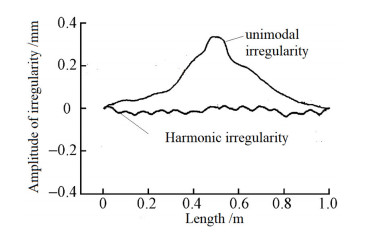
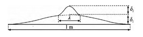
[30]	S. Ma, L. Gao, X. B. Liu, J. Tu, J. L. Sun, Y. W. Wei, Measurement and analysis of unevenness of welded joints of ballastless track for passenger-freight common line (in Chinese), Railway Eng., 59 (2019), 152–156.
[31]	J. M. Gao, W. M. Zhai, Dynamic effect and safety limits of rail weld irregularity on high-speed railways, Sci. Sin. Technol., 44 (2014), 697–706. https://doi.org/10.1360/N092014-00081 doi: 10.1360/N092014-00081
[32]	TB/T3276−2011, Rail for high-speed railway, 2011.
[33]	G. Q. Cui, Research on reasonable stiffness of double block ballastless track (in Chinese), Railway Eng., (2009), 93–96.
[34]	S. J. Li, X. X. Ma, Application of the vibration measurement system in dynamic parameter measurement (in Chinese), Res. Explor. Lab., 38 (2019), 58–61.
[35]	W. T. Xu, Y. H. Zhang, G. W. Tang, G. J. Pan, Variable damping characteristics of Magnesium alloys and its Dynamic Analysis Method, Appl. Math. Mech., 41 (2020), 1297–1310.
[36]	D. Chen, Stiffness Analysis of Railway Vehicle Air Spring, Master's thesis, Southwest Jiaotong University, 2011.
[37]	W. J. Yin, Y. Han, S. P. Yang, Dynamic analysis of air spring suspension system under forced vibration (in Chinese), China J. Highway Transp., 19 (2006), 117–121. https://doi.org/10.19721/j.cnki.1001-7372.2006.03.022 doi: 10.19721/j.cnki.1001-7372.2006.03.022
[38]	Q. Y. Zhou, The Hundred-year development history of rail type and measuring length in China (in Chinese), China Railway, 2022 (2022), 42–46. https://doi.org/10.19549/j.issn.1001-683x.2021.08.18.001 doi: 10.19549/j.issn.1001-683x.2021.08.18.001
[39]	J. Zeng, J. Y. Zhang, Z. Y. Shen, Hopf bifurcation and nonlinear oscillations in railway vehicle systems, Veh. Syst. Dyn., 33 (1999), 552–565. https://doi.org/10.1080/00423114.1999.12063111 doi: 10.1080/00423114.1999.12063111
[40]	J. Zeng, W. H. Zhang, H. Y. Dai, X. J. Wu, Z. Y. Shen, Hunting instability analysis and H∞ controlled stabilizer design for high-speed railway passenger car, Veh. Syst. Dyn., 29 (1998), 655–668. https://doi.org/10.1080/00423119808969593 doi: 10.1080/00423119808969593
[41]	G. W. Luo, J. H. Xie, Periodic Motion and Bifurcation of Collisional Vibration System, Science Press, 2004.

This article has been cited by:

Ching-Lung Lin, Hongyu Liu, Catharine W. K. Lo, Uniqueness principle for fractional (non)-coercive anisotropic polyharmonic operators and applications to inverse problems, 2024, 0, 1930-8337, 0, 10.3934/ipi.2024054

Reader Comments

Your name:*

Email:*
© 2023 the Author(s), licensee AIMS Press. This is an open access article distributed under the terms of the Creative Commons Attribution License (http://creativecommons.org/licenses/by/4.0)