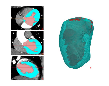
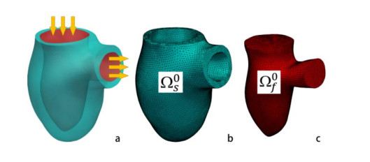
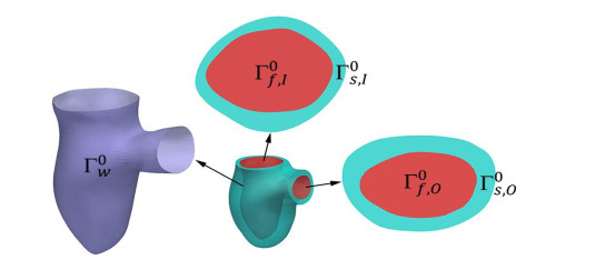
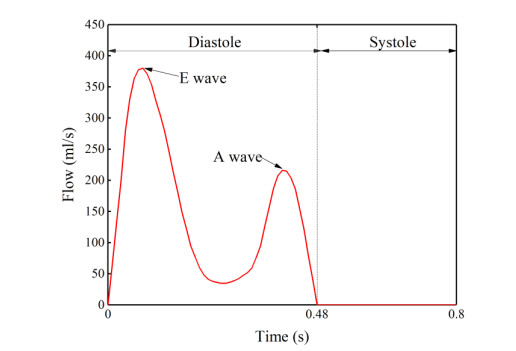
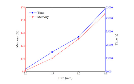
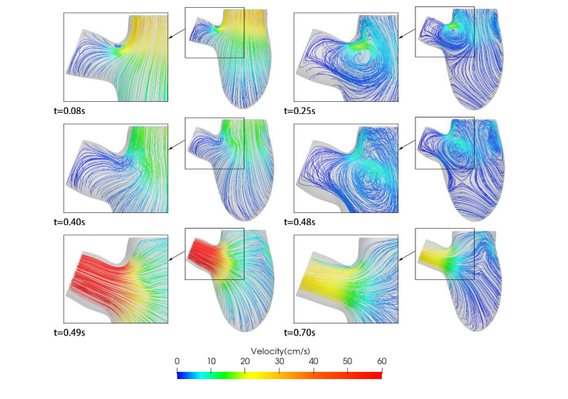
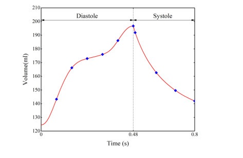
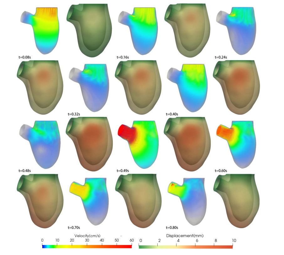
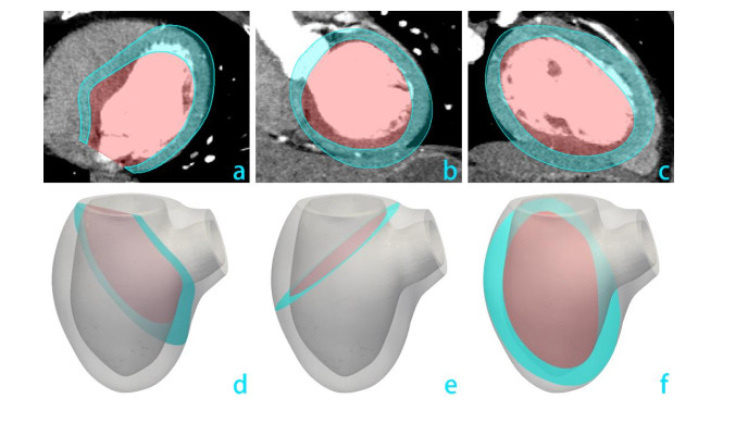
In this paper, we propose a scalable parallel algorithm for simulating the cardiac fluid-structure interactions (FSI) of a patient-specific human left ventricle. It provides an efficient forward solver to deal with the induced sub-problems in solving an inverse problem that can be used to quantify the interested parameters. The FSI between the blood flow and the myocardium is described in an arbitrary Lagrangian-Eulerian (ALU) framework, in which the velocity and stress are assumed being continuous across the fluid-structure interface. The governing equations are discretized by using a finite element method and a fully implicit backward Eulerian formula, and the resulting algebraic system is solved by using a parallel Newton-Krylov-Schwarz algorithm. We numerically show that the algorithm is robust with respect to multiple model parameters and scales well up to 2300 processor cores. The ability of the proposed method to produce qualitatively true prediction is also demonstrated via comparing the simulation results with the clinic data.
Citation: Yujia Chang, Yi Jiang, Rongliang Chen. A parallel domain decomposition algorithm for fluid-structure interaction simulations of the left ventricle with patient-specific shape[J]. Electronic Research Archive, 2022, 30(9): 3377-3396. doi: 10.3934/era.2022172
In this paper, we propose a scalable parallel algorithm for simulating the cardiac fluid-structure interactions (FSI) of a patient-specific human left ventricle. It provides an efficient forward solver to deal with the induced sub-problems in solving an inverse problem that can be used to quantify the interested parameters. The FSI between the blood flow and the myocardium is described in an arbitrary Lagrangian-Eulerian (ALU) framework, in which the velocity and stress are assumed being continuous across the fluid-structure interface. The governing equations are discretized by using a finite element method and a fully implicit backward Eulerian formula, and the resulting algebraic system is solved by using a parallel Newton-Krylov-Schwarz algorithm. We numerically show that the algorithm is robust with respect to multiple model parameters and scales well up to 2300 processor cores. The ability of the proposed method to produce qualitatively true prediction is also demonstrated via comparing the simulation results with the clinic data.

| [1] |
M. Nash, P. Hunter, Computational mechanics of the heart, J. Elasticity, 61 (2000), 113-141. https://doi.org/10.1023/A:1011084330767 doi: 10.1023/A:1011084330767

|
| [2] |
D. Kass, C.-H. Chen, C. Curry, M. Talbot, R. Berger, B. Fetics, et al., Improved left ventricular mechanics from acute VDD pacing in patients with dilated cardiomyopathy and ventricular conduction delay, Circulation, 99 (1999), 1567-1573. https://doi.org/10.1161/01.CIR.99.12.1567 doi: 10.1161/01.CIR.99.12.1567
|
| [3] |
S. N. Doost, D. Ghista, B. Su, L. Zhong, Y. S. Morsi, Heart blood flow simulation: a perspective review, Biomed. Eng. Online, 15 (2016), 1-28. https://doi.org/10.1186/s12938-016-0224-8 doi: 10.1186/s12938-016-0224-8
|
| [4] |
R. Mittal, J. H. Seo, V. Vedula, Y. J. Choi, H. Liu, H. H. Huang, et al., Computational modeling of cardiac hemodynamics: Current status and future outlook, J. Comput. Phys., 305 (2016), 1065-1082. https://doi.org/10.1016/j.jcp.2015.11.022 doi: 10.1016/j.jcp.2015.11.022
|
| [5] |
J. Li, J. M. Melenk, B. Wohlmuth, J. Zou, Optimal a priori estimates for higher order finite elements for elliptic interface problems, Appl. Numer. Math., 60 (2010), 19-37. https://doi.org/10.1016/j.apnum.2009.08.005 doi: 10.1016/j.apnum.2009.08.005
|
| [6] |
J. Li, J. Xie, J. Zou, An adaptive finite element reconstruction of distributed fluxes, Inverse Probl., 27 (2011), 075009. https://doi.org/10.1088/0266-5611/27/7/075009 doi: 10.1088/0266-5611/27/7/075009
|
| [7] |
X. Cao, H. Diao, J. Li, Some recent progress on inverse scattering problems within general polyhedral geometry, Electron. Res. Arch., 29 (2021), 1753-1782. https://doi.org/10.3934/era.2020090 doi: 10.3934/era.2020090
|
| [8] |
J. Li, H. Liu, H. Sun, On an inverse elastic wave imaging scheme for nearly incompressible materials, IMA J. Appl. Math., 84 (2018), 229-257. https://doi.org/10.1093/imamat/hxy056 doi: 10.1093/imamat/hxy056
|
| [9] |
H. Diao, H. Liu, L. Wang, On generalized Holmgren's principle to the Lame operator with applications to inverse elastic problems, Calc. Var. Partial Differ. Equ., 59 (2020), 179. https://doi.org/10.1007/s00526-020-01830-5 doi: 10.1007/s00526-020-01830-5
|
| [10] |
H. Diao, H. Liu, B. Sun, On a local geometric property of the generalized elastic transmission eigenfunctions and application, Inverse Probl., 37 (2021), 105015. https://doi.org/10.1088/1361-6420/ac23c2 doi: 10.1088/1361-6420/ac23c2
|
| [11] |
X. Wang, Y. Guo, S. Bousba, Direct imaging for the moment tensor point sources of elastic waves, J. Comput. Phys., 448 (2022), 110731. https://doi.org/10.1016/j.jcp.2021.110731 doi: 10.1016/j.jcp.2021.110731
|
| [12] |
H. Li, H. Liu, J. Zou, Minnaert resonances for bubbles in soft elastic materials, SIAM J. Appl. Math., 82 (2022), 119-141. https://doi.org/10.1137/21M1400572 doi: 10.1137/21M1400572
|
| [13] |
H. Liu, W.-Y. Tsui, A. Wahab, X. Wang, Three-dimensional elastic scattering coefficients and enhancement of the elastic near cloaking, J. Elasticity, 143 (2021), 111-146. https://doi.org/10.1007/s10659-020-09807-3 doi: 10.1007/s10659-020-09807-3
|
| [14] |
Y. Deng, H. Li, H. Liu, On spectral properties of Neuman-Poincare operator and plasmonic resonances in 3D elastostatics, J. Spectr. Theory, 9 (2019), 767-789. https://doi.org/10.4171/JST/262 doi: 10.4171/JST/262
|
| [15] |
H. Li, J. Li, H. Liu, On novel elastic structures inducing polariton resonances with finite frequencies and cloaking due to anomalous localized resonances, J. Math. Pures Appl., 120 (2018), 195-219. https://doi.org/10.1016/j.matpur.2018.06.014 doi: 10.1016/j.matpur.2018.06.014
|
| [16] |
H. Li, H. Liu, On anomalous localized resonance for the elastostatic system, SIAM J. Math. Anal., 48 (2016), 3322-3344. https://doi.org/10.1137/16M1059023 doi: 10.1137/16M1059023
|
| [17] |
E. H. Dowell, K. C. Hall, Modeling of fluid-structure interaction, Annu. Rev. Fluid Mech., 33 (2001), 445-490. https://doi.org/10.1146/annurev.fluid.33.1.445 doi: 10.1146/annurev.fluid.33.1.445
|
| [18] |
G. Hou, J. Wang, A. Layton, Numerical methods for fluid-structure interaction---a review, Commun. Comput. Phys., 12 (2012), 337-377. https://doi.org/10.4208/cicp.291210.290411s doi: 10.4208/cicp.291210.290411s
|
| [19] |
F. Jiang, Stabilizing effect of elasticity on the motion of viscoelastic/elastic fluids, Electron. Res. Arch., 29, 2021, 4051-4074. https://doi.org/10.3934/era.2021071 doi: 10.3934/era.2021071
|
| [20] |
C. Hirt, A. Anthony, J. L. Cook, An arbitrary Lagrangian-Eulerian computing method for all flow speeds, J. Comput. Phys., 14 (1974), 227-253. https://doi.org/10.1016/0021-9991(74)90051-5 doi: 10.1016/0021-9991(74)90051-5
|
| [21] |
M.-C. Hsu, D. Kamensky, Y. Bazilevs, M. S. Sacks, T. JR Hughes, Fluid-structure interaction analysis of bioprosthetic heart valves: significance of arterial wall deformation, Comput. Mech., 54 (2014), 1055-1071. https://doi.org/10.1007/s00466-014-1059-4 doi: 10.1007/s00466-014-1059-4
|
| [22] |
C. Peskin, Flow patterns around heart valves: A numerical method, J. Comput. Phys., 10 (1972), 252-271. https://doi.org/10.1016/0021-9991(72)90065-4 doi: 10.1016/0021-9991(72)90065-4
|
| [23] |
F. Sotiropoulos, X. Yang, Immersed boundary methods for simulating fluid-structure interaction, Prog. Aerosp. Sci., 65 (2014), 1-21. https://doi.org/10.1016/j.paerosci.2013.09.003 doi: 10.1016/j.paerosci.2013.09.003
|
| [24] |
W. Kim, H. Choi, Immersed boundary methods for fluid-structure interaction: A review, Int. J. Heat Fluid Flow, 75 (2019), 301-309. https://doi.org/10.1016/j.ijheatfluidflow.2019.01.010 doi: 10.1016/j.ijheatfluidflow.2019.01.010
|
| [25] |
D. Jones, X. Zhang, A conforming-nonconforming mixed immersed finite element method for unsteady stokes equations with moving interfaces, Electron. Res. Arch., 29, (2021), 3171-3191. https://doi.org/10.3934/era.2021032 doi: 10.3934/era.2021032
|
| [26] |
D. Boffi, L. Gastaldi, A finite element approach for the immersed boundary method, Comput. Struct., 81 (2003), 491-501. https://doi.org/10.1016/S0045-7949(02)00404-2 doi: 10.1016/S0045-7949(02)00404-2
|
| [27] |
B. E. Griffith, X. Luo, Hybrid finite difference/finite element immersed boundary method, Int. J. Numer. Method Biomed. Eng., 33 (2017), e2888. https://doi.org/10.1002/cnm.2888 doi: 10.1002/cnm.2888
|
| [28] |
H. Watanabe, T. Hisada, S. Sugiura, J. Okada, H. Fukunari, Computer Simulation of Blood Flow, Left Ventricular Wall Motion and Their Interrelationship by Fluid-Structure Interaction Finite Element Method, JSME Int. J. C-Mech. SY, 45 (2002), 1003-1021. https://doi.org/10.1299/jsmec.45.1003 doi: 10.1299/jsmec.45.1003
|
| [29] |
H. Watanabe, S. Sugiura, H. Kafuku, T. Hisada, Multiphysics Simulation of Left Ventricular Filling Dynamics Using Fluid-Structure Interaction Finite Element Method, Biophys. J., 87 (2004), 2074-2085. https://doi.org/10.1529/biophysj.103.035840 doi: 10.1529/biophysj.103.035840
|
| [30] | M. Doyle, S. Tavoularis, Y. Bourgault, Application of Parallel Processing to the Simulation of Heart Mechanics, International Symposium on High Performance Computing Systems and Applications, Springer, Berlin, Heidelberg, 2009. https://doi.org/10.1007/978-3-642-12659-8_3 |
| [31] |
D. Nordsletten, M. McCormick, P. J. Kilner, D. Kay, N. P. Smith, Fluid-solid coupling for the investigation of diastolic and systolic human left ventricular function, Int. J. Numer. Methods Biomed. Eng., 27 (2011), 1017-1039. https://doi.org/10.1002/cnm.1405 doi: 10.1002/cnm.1405
|
| [32] |
H. Gao, D. Carrick, C. Berry, B. Griffith, X. Luo, Dynamic finite-strain modelling of the human left ventricle in health and disease using an immersed boundary-finite element method, IMA J. Appl. Math., 79 (2014), 978-1010. https://doi.org/10.1093/imamat/hxu029 doi: 10.1093/imamat/hxu029
|
| [33] |
H. Gao, H. Wang, C. Berry, X. Luo, B. Griffith, Quasi-static image-based immersed boundary-finite element model of left ventricle under diastolic loading, Int. J. Numer. Methods Biomed. Eng., 30 (2014), 1199-1222. https://doi.org/10.1002/cnm.2652 doi: 10.1002/cnm.2652
|
| [34] |
Y. Wu, X.-C. Cai, A fully implicit domain decomposition based ALE framework for three-dimensional fluid-structure interaction with application in blood flow computation, J. Comput. Phys., 258 (2014), 524-537. https://doi.org/10.1016/j.jcp.2013.10.046 doi: 10.1016/j.jcp.2013.10.046
|
| [35] |
L. Franca, S. Frey, Stabilized finite element methods: Ⅱ. The incompressible Navier-Stokes equations, Comput. Methods Appl. Mech. Eng., 99 (1992), 209-233. https://doi.org/10.1016/0045-7825(92)90041-H doi: 10.1016/0045-7825(92)90041-H
|
| [36] | W. Ames, W. Rheinboldt, A. Jeffrey, Numerical Methods Partial Differential Equation, Second Edition, Academic Press, 1977. |
| [37] |
X.-C. Cai, M. Sarkis, A Restricted Additive Schwarz Preconditioner for General Sparse Linear Systems, SIAM J. Sci. Comput., 21 (1999), 792-797. https://doi.org/10.1137/S106482759732678X doi: 10.1137/S106482759732678X
|
Figures(16) / Tables(7)
Yujia Chang, Yi Jiang, Rongliang Chen. A parallel domain decomposition algorithm for fluid-structure interaction simulations of the left ventricle with patient-specific shape[J]. Electronic Research Archive, 2022, 30(9): 3377-3396. doi: 10.3934/era.2022172


 DownLoad: