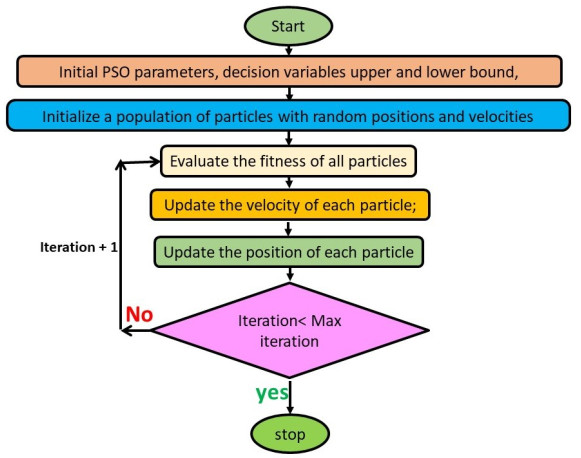
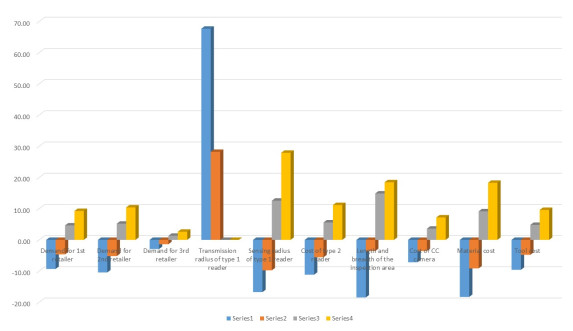
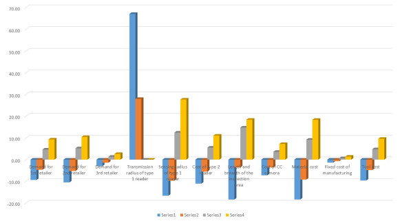
The proposed study described the application of innovative technology to solve the issues in a supply chain model due to the players' unreliability. The unreliable manufacturer delivers a percentage of the ordered quantity to the retailer, which causes shortages. At the same time, the retailer provides wrong information regarding the amount of the sales of the product. Besides intelligent technology, a single setup multiple unequal increasing delivery transportation policy is applied in this study to reduce the holding cost of the retailer. A consumed fuel and electricity-dependent carbon emission cost are used for environmental sustainability. Since the industries face problems with smooth functioning in each of its steps for unreliable players, the study is proposed to solve the unpredictable player problem in the supply chain. The robust distribution approach is utilized to overcome the situation of unknown lead time demand. Two metaheuristic optimization techniques, genetic algorithm (GA) and particle swarm optimization (PSO) are used to optimize the total cost. From the numerical section, it is clear the PSO is $ 0.32 $ % more beneficial than GA to obtain the minimum total cost of the supply chain. The discussed case studies show that the applied single-setup-multi-unequal-increasing delivery policy is $ 0.62 $ % beneficial compared to the single-setup-single-delivery policy and $ 0.35 $ % beneficial compared to the single-setup-multi-delivery policy. The sensitivity analysis with graphical representation is provided to explain the result clearly.
Citation: Soumya Kanti Hota, Santanu Kumar Ghosh, Biswajit Sarkar. Involvement of smart technologies in an advanced supply chain management to solve unreliability under distribution robust approach[J]. AIMS Environmental Science, 2022, 9(4): 461-492. doi: 10.3934/environsci.2022028
The proposed study described the application of innovative technology to solve the issues in a supply chain model due to the players' unreliability. The unreliable manufacturer delivers a percentage of the ordered quantity to the retailer, which causes shortages. At the same time, the retailer provides wrong information regarding the amount of the sales of the product. Besides intelligent technology, a single setup multiple unequal increasing delivery transportation policy is applied in this study to reduce the holding cost of the retailer. A consumed fuel and electricity-dependent carbon emission cost are used for environmental sustainability. Since the industries face problems with smooth functioning in each of its steps for unreliable players, the study is proposed to solve the unpredictable player problem in the supply chain. The robust distribution approach is utilized to overcome the situation of unknown lead time demand. Two metaheuristic optimization techniques, genetic algorithm (GA) and particle swarm optimization (PSO) are used to optimize the total cost. From the numerical section, it is clear the PSO is $ 0.32 $ % more beneficial than GA to obtain the minimum total cost of the supply chain. The discussed case studies show that the applied single-setup-multi-unequal-increasing delivery policy is $ 0.62 $ % beneficial compared to the single-setup-single-delivery policy and $ 0.35 $ % beneficial compared to the single-setup-multi-delivery policy. The sensitivity analysis with graphical representation is provided to explain the result clearly.

| [1] |
Frank AG, Dalenogare LS, Ayala NF (2019) Industry 4.0 technologies: Implementation patterns in manufacturing companies. International Journal of Production Economics 210: 15–26. https://doi.org/10.1016/j.ijpe.2019.01.004 doi: 10.1016/j.ijpe.2019.01.004

|
| [2] |
Bueno AF, Godinho Filho M, Frank AG (2020) Smart production planning and control in the Industry 4.0 context: A systematic literature review. Computers & Industrial Engineering 149: 106774. https://doi.org/10.1016/j.cie.2020.106774 doi: 10.1016/j.cie.2020.106774
|
| [3] |
Sardar SK, Sarkar B, Kim B (2021) Integrating Machine Learning, Radio Frequency Identification, and Consignment Policy for Reducing Unreliability in Smart Supply Chain Management Processes 9: 247. https://doi.org/10.3390/pr9020247 doi: 10.3390/pr9020247
|
| [4] |
Tseng ML, Tran TPT, Ha HM, et al. (2021) Sustainable industrial and operation engineering trends and challenges Toward Industry 4.0: A data driven analysis. Journal of Industrial and Production Engineering 38: 581–598. https://doi.org/10.1080/21681015.2021.1950227 doi: 10.1080/21681015.2021.1950227
|
| [5] |
Sarkar M, Pan L, Dey BK, et al. (2020) Does the Autonomation Policy Really Help in a Smart Production System for Controlling Defective Production? Mathematics 8: 1142. https://doi.org/10.3390/math8071142 doi: 10.3390/math8071142
|
| [6] |
Sarkar M, Chung BD (2021) Effect of Renewable Energy to Reduce Carbon Emissions under a Flexible Production System: A Step Toward Sustainability. Energies 14: 215. https://doi.org/10.3390/en14010215 doi: 10.3390/en14010215
|
| [7] |
Jwo JS, Lin CS, Lee CH (2021) Smart technology–driven aspects for human-in-the-loop smart manufacturing. The International Journal of Advanced Manufacturing Technology 114: 1741–1752. https://doi.org/10.1007/s00170-021-06977-9 doi: 10.1007/s00170-021-06977-9
|
| [8] |
El Cadi AA, Gharbi A, Dhouib K, et al. (2021) Joint production and preventive maintenance controls for unreliable and imperfect manufacturing systems. Journal of Manufacturing Systems 58: 263–279. https://doi.org/10.1016/j.jmsy.2020.12.003 doi: 10.1016/j.jmsy.2020.12.003
|
| [9] |
Sarkar B, Guchhait R, Sarkar M, et al. (2019) How does an industry manage the optimum cash flow within a smart production system with the carbon footprint and carbon emission under logistics framework? International Journal of Production Economics 213: 243–257. https://doi.org/10.1016/j.ijpe.2019.03.012 doi: 10.1016/j.ijpe.2019.03.012
|
| [10] |
Roy MD, Sana SS (2021) Production rate and lot-size dependent lead time reduction strategies in a supply chain model with stochastic demand, controllable setup cost and trade-credit financing. RAIRO: Recherche Opérationnelle 55: 1469. https://doi.org/10.1051/ro/2020112 doi: 10.1051/ro/2020112
|
| [11] |
Jeong H, Karim RA, Sieverding HL, et al. (2021) An Application of GIS-Linked Biofuel Supply Chain Optimization Model for Various Transportation Network Scenarios in Northern Great Plains (NGP), USA. BioEnergy Research 14: 612–622. https://doi.org/10.1007/s12155-020-10223-7 doi: 10.1007/s12155-020-10223-7
|
| [12] |
Sedehzadeh S, Seifbarghy M (2021) Redesigning a fast-moving consumer goods supply chain considering social responsibility and logistical restrictions: case study in an Iranian food company. Environmental Science and Pollution Research 2021: 1–16. https://doi.org/10.1007/s11356-021-14760-2 doi: 10.1007/s11356-021-14760-2
|
| [13] |
Guchhait R, Pareek S, Sarkar B (2019) How Does a Radio Frequency Identification Optimize the Profit in an Unreliable Supply Chain Management? Mathematics 7: 490. https://doi.org/10.3390/math7060490 doi: 10.3390/math7060490
|
| [14] |
Hoque M (2020) A manufacturer-buyers integrated inventory model with various distributions of lead times of delivering equal-sized batches of a lot. Computers & Industrial Engineering 145: 106516. https://doi.org/10.1016/j.cie.2020.106516 doi: 10.1016/j.cie.2020.106516
|
| [15] |
Sarkar B, Saren S, Sinha D, et al. (2015) Effect of unequal lot sizes, variable setup cost, and carbon emission cost in a supply chain model. Mathematical Problems in Engineering 2015. https://doi.org/10.1155/2015/469486 doi: 10.1155/2015/469486
|
| [16] |
Hota SK, Sarkar B, Ghosh SK (2020) Effects of unequal lot size and variable transportation in unreliable supply chain management. Mathematics 8: 357. https://doi.org/10.3390/math8030357 doi: 10.3390/math8030357
|
| [17] |
Ai Y, Xu Y (2021) Strategic sourcing in forward and spot markets with reliable and unreliable suppliers. International Journal of Production Research 59: 926–941. https://doi.org/10.1080/00207543.2020.1711987 doi: 10.1080/00207543.2020.1711987
|
| [18] |
Giri BC, Majhi JK, Chaudhuri K (2021) Coordination mechanisms of a three-layer supply chain under demand and supply risk uncertainties. RAIRO-Operations Research 55: S2593–S2617. https://doi.org/10.1051/ro/2020101 doi: 10.1051/ro/2020101
|
| [19] |
Hlioui R, Gharbi A, Hajji A (2017) Joint supplier selection, production and replenishment of an unreliable manufacturing-oriented supply chain. International Journal of Production Economics. 187: 53–67. https://doi.org/10.1016/j.ijpe.2017.02.004 doi: 10.1016/j.ijpe.2017.02.004
|
| [20] | Scarf H (1958) A min-max solution of an inventory problem. Studies in the mathematical theory of inventory and production |
| [21] |
Pal B, Adhikari S (2022) Optimal strategies for members in a two-echelon supply chain over a safe period under random machine hazards with backlogging. Journal of Industrial and Production Engineering 2022: 1–18. https://doi.org/10.1080/21681015.2021.2001767 doi: 10.1080/21681015.2021.2001767
|
| [22] |
Elfarouk O, Wong KY, Wong WP (2022) Multi-objective optimization for multi-echelon, multi-product, stochastic sustainable closed-loop supply chain. Journal of Industrial and Production Engineering 39: 109–127. https://doi.org/10.1080/21681015.2021.1963338 doi: 10.1080/21681015.2021.1963338
|
| [23] |
Chen Y, Feng Q, Senior Member I, et al. (2021) Modeling and analyzing RFID Generation-2 under unreliable channels. Journal of Network and Computer Applications 178: 102937. https://doi.org/10.1016/j.jnca.2020.102937 doi: 10.1016/j.jnca.2020.102937
|
| [24] |
Entezaminia A, Gharbi A, Ouhimmou M (2021) A joint production and carbon trading policy for unreliable manufacturing systems under cap-and-trade regulation. Journal of Cleaner Production 293: 125973. https://doi.org/10.1016/j.jclepro.2021.125973 doi: 10.1016/j.jclepro.2021.125973
|
| [25] |
Romero-Silva R, Shaaban S, Marsillac E, et al. (2021) The Impact of Unequal Processing Time Variability on Reliable and Unreliable Merging Line Performance. International Journal of Production Economics 2021: 108108. https://doi.org/10.1016/j.ijpe.2021.108108 doi: 10.1016/j.ijpe.2021.108108
|
| [26] |
Sardar SK, Sarkar B (2020) How Does Advanced Technology Solve Unreliability Under Supply Chain Management Using Game Policy? Mathematics 8 :1191. https://doi.org/10.3390/math8071191 doi: 10.3390/math8071191
|
| [27] |
Sarkar B, Omair M, Kim N (2020) A cooperative advertising collaboration policy in supply chain management under uncertain conditions. Applied Soft Computing 88 :105948. https://doi.org/10.1016/j.asoc.2019.105948 doi: 10.1016/j.asoc.2019.105948
|
| [28] |
Park K, Lee K (2016) Distribution-robust single-period inventory control problem with multiple unreliable suppliers. OR spectrum 38 :949–966. https://doi.org/10.1007/s00291-016-0440-4 doi: 10.1007/s00291-016-0440-4
|
| [29] |
Ullah M, Sarkar B (2020) Recovery-channel selection in a hybrid manufacturing-remanufacturing production model with RFID and product quality. International Journal of Production Economics 219: 360–374. https://doi.org/10.1016/j.ijpe.2019.07.017 doi: 10.1016/j.ijpe.2019.07.017
|
| [30] |
Dalenogare LS, Benitez GB, Ayala NF, et al. (2018) The expected contribution of Industry 4.0 technologies for industrial performance. International Journal of Production Economics 204: 383–394. https://doi.org/10.1016/j.ijpe.2018.08.019 doi: 10.1016/j.ijpe.2018.08.019
|
| [31] |
Wang S, Wan J, Zhang D, et al. (2016) Towards smart factory for industry 4.0: a self-organized multi-agent system with big data based feedback and coordination. Computer Networks 101: 158–168. https://doi.org/10.1016/j.comnet.2015.12.017 doi: 10.1016/j.comnet.2015.12.017
|
| [32] |
Chen B, Wan J, Shu L, et al. (2017) Smart factory of industry 4.0: Key technologies, application case, and challenges. Ieee Access 6: 6505–6519. https://doi.org/10.1109/ACCESS.2017.2783682 doi: 10.1109/ACCESS.2017.2783682
|
| [33] |
Dey BK, Pareek S, Tayyab M, et al. (2021) Autonomation policy to control work-in-process inventory in a smart production system. International Journal of Production Research 59: 1258–1280. https://doi.org/10.1080/00207543.2020.1722325 doi: 10.1080/00207543.2020.1722325
|
| [34] |
Bhuniya S, Pareek S, Sarkar B, et al. (2021) A Smart Production Process for the Optimum Energy Consumption with Maintenance Policy under a Supply Chain Management. Processes 9: 19. https://doi.org/10.3390/pr9010019 doi: 10.3390/pr9010019
|
| [35] |
Sarkar M, Sarkar B (2019) Optimization of safety stock under controllable production rate and energy consumption in an automated smart production management. Energies 12: 2059. https://doi.org/10.3390/en12112059 doi: 10.3390/en12112059
|
| [36] |
Goyal SK (1988) "A joint economic-lot-size model for purchaser and vendor": A comment. Decision sciences 19:236–241. doi: 10.1111/j.1540-5915.1988.tb00264.x
|
| [37] |
Hoque M (2013) A manufacturer–buyer integrated inventory model with stochastic lead times for delivering equal-and/or unequal-sized batches of a lot. Computers & operations research 40: 2740–2751. https://doi.org/10.1016/j.cor.2013.05.008 doi: 10.1016/j.cor.2013.05.008
|
| [38] |
Hariga M, Gumus M, Daghfous A (2014) Storage constrained vendor managed inventory models with unequal shipment frequencies. Omega 48: 94–106. https://doi.org/10.1016/j.omega.2013.11.003 doi: 10.1016/j.omega.2013.11.003
|
| [39] |
Garai A, Sarkar B (2022) Economically independent reverse logistics of customer-centric closed-loop supply chain for herbal medicines and biofuel. Journal of Cleaner Production 334: 129977. https://doi.org/10.1016/j.jclepro.2021.129977 doi: 10.1016/j.jclepro.2021.129977
|
| [40] |
Sarkar B, Debnath A, Chiu AS, et al. (2022) Circular economy-driven two-stage supply chain management for nullifying waste. Journal of Cleaner Production 339: 130513. https://doi.org/10.1016/j.jclepro.2022.130513 doi: 10.1016/j.jclepro.2022.130513
|
| [41] |
Sarkar B, Bhuniya S (2022) A sustainable flexible manufacturing–remanufacturing model with improved service and green investment under variable demand. Expert Systems with Applications 202: 117154. https://doi.org/10.1016/j.eswa.2022.117154 doi: 10.1016/j.eswa.2022.117154
|
| [42] |
Choi SB, Dey BK, Kim SJ, et al. (2022) Intelligent servicing strategy for an online-to-offline (O2O) supply chain under demand variability and controllable lead time. RAIRO-Operations Research 2022 https://doi.org/10.1051/ro/2022026 doi: 10.1051/ro/2022026
|
| [43] |
Sarkar B, Ullah M, Sarkar M (2022) Environmental and economic sustainability through innovative green products by remanufacturing. Journal of Cleaner Production 332: 129813. https://doi.org/10.1016/j.jclepro.2021.129813 doi: 10.1016/j.jclepro.2021.129813
|
| [44] |
Majumder A, Jaggi CK, Sarkar B (2018) A multi-retailer supply chain model with backorder and variable production cost. RAIRO-Operations Research 52: 943–954. https://doi.org/10.1051/ro/2017013 doi: 10.1051/ro/2017013
|
| [45] |
Tang S, Wang W, Cho S, et al. (2018) Reducing emissions in transportation and inventory management:(R, Q) Policy with considerations of carbon reduction European Journal of Operational Research 269: 327–340. https://doi.org/10.1016/j.ejor.2017.10.010 doi: 10.1016/j.ejor.2017.10.010
|
| [46] |
Bhuniya S, Sarkar B, Pareek S (2019) Multi-product production system with the reduced failure rate and the optimum energy consumption under variable demand Mathematics 7: 465. https://doi.org/10.3390/math7050465 doi: 10.3390/math7050465
|
| [47] |
Mishra M, Hota SK, Ghosh SK, et al. (2020) Controlling Waste and Carbon Emission for a Sustainable Closed-Loop Supply Chain Management under a Cap-and-Trade Strategy. Mathematics 8: 466. https://doi.org/10.3390/math8040466 doi: 10.3390/math8040466
|
| [48] |
Manna AK, Mondal R, Akbar Shaikh A, et al. (2021) Single-manufacturer and multi-retailer supply chain model with pre-payment based partial free transportation. RAIRO-Operations Research 55: 1063–1076. https://doi.org/10.1051/ro/2021053 doi: 10.1051/ro/2021053
|
| [49] |
Lin YJ (2008) Minimax distribution free procedure with backorder price discount. International Journal of Production Economics 111: 118–128. https://doi.org/10.1016/j.ijpe.2006.11.016 doi: 10.1016/j.ijpe.2006.11.016
|
| [50] |
Moon I, Choi S (1998) TECHNICAL NOTEA note on lead time and distributional assumptions in continuous review inventory models. Computers & Operations Research 25: 1007–1012. https://doi.org/10.1016/S0305-0548(97)00103-2 doi: 10.1016/S0305-0548(97)00103-2
|
| [51] |
Centobelli P, Cerchione R, Del Vecchio P, et al. (2021) Blockchain technology for bridging trust, traceability and transparency in circular supply chain. Information & Management 2021: 103508 https://doi.org/10.1016/j.im.2021.103508 doi: 10.1016/j.im.2021.103508
|
| [52] |
Kshetri N (2021) Blockchain and sustainable supply chain management in developing countries. International Journal of Information Management 60: 102376. https://doi.org/10.1016/j.ijinfomgt.2021.102376 doi: 10.1016/j.ijinfomgt.2021.102376
|
| [53] |
Shen C, Pena-Mora F (2018) Blockchain for cities—a systematic literature review. Ieee Access 6: 76787–76819. https://doi.org/10.1109/ACCESS.2018.2880744 doi: 10.1109/ACCESS.2018.2880744
|
| [54] |
Centobelli P, Cerchione R, Del Vecchio P, et al. (2021) Blockchain technology design in accounting: Game changer to tackle fraud or technological fairy tale? Accounting, Auditing & Accountability Journal 2021. https://doi.org/10.1108/AAAJ-10-2020-4994 doi: 10.1108/AAAJ-10-2020-4994
|
| [55] | Zhang H, Hou JC (2005) Maintaining sensing coverage and connectivity in large sensor networks. Ad Hoc Sens Wirel Networks 1: 89–124. |
| [56] |
Hefeeda M, Ahmadi H (2007) A probabilistic coverage protocol for wireless sensor networks. 2007 IEEE International Conference on Network Protocols 2007: 41–50. https://doi.org/10.1109/ICNP.2007.4375835 doi: 10.1109/ICNP.2007.4375835
|
| [57] |
Hota SK, Ghosh SK, Sarkar B (2022) A solution to the transportation hazard problem in a supply chain with an unreliable manufacturer AIMS Environmental Science 9: 354–380. https://doi.org/10.3934/environsci.2022023 doi: 10.3934/environsci.2022023
|
Figures(8) / Tables(3)

Soumya Kanti Hota, Santanu Kumar Ghosh, Biswajit Sarkar. Involvement of smart technologies in an advanced supply chain management to solve unreliability under distribution robust approach[J]. AIMS Environmental Science, 2022, 9(4): 461-492. doi: 10.3934/environsci.2022028


 DownLoad: