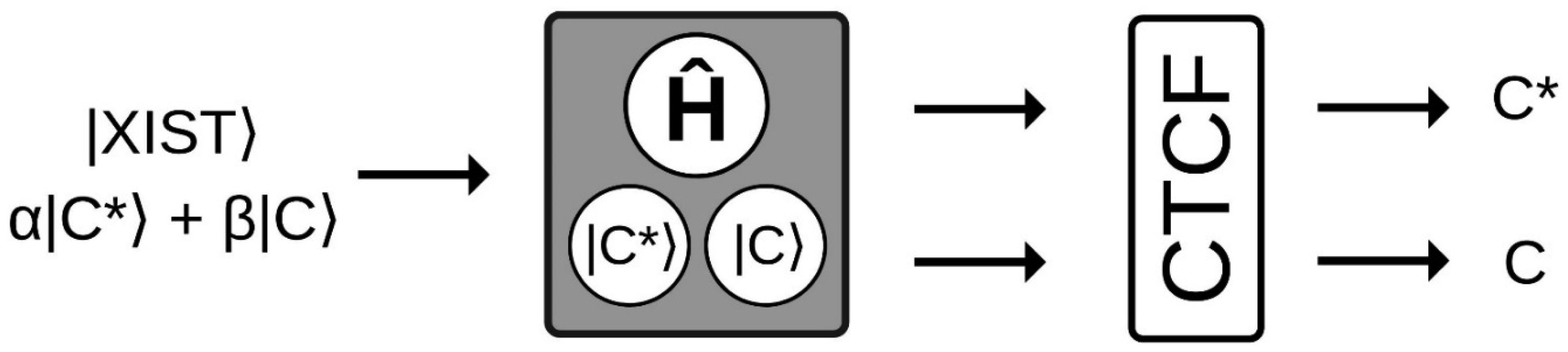
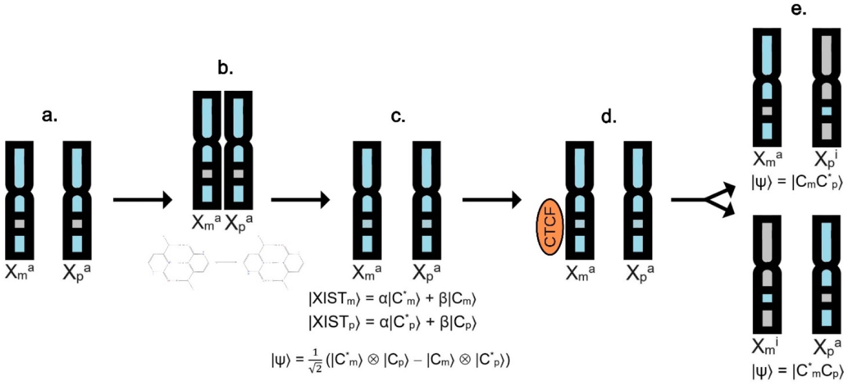
The X chromosome inactivation is an essential mechanism in mammals' development, that despite having been investigated for 60 years, many questions about its choice process have yet to be fully answered. Therefore, a theoretical model was proposed here for the first time in an attempt to explain this puzzling phenomenon through a quantum mechanical approach. Based on previous data, this work theoretically demonstrates how a shared delocalized proton at a key base pair position could explain the random, instantaneous, and mutually exclusive nature of the choice process in X chromosome inactivation. The main purpose of this work is to contribute to a comprehensive understanding of the X inactivation mechanism with a model proposal that can complement the existent ones, along with introducing a quantum mechanical approach that could be applied to other cell differentiation mechanisms.
Citation: Rodrigo Lobato. A quantum mechanical approach to random X chromosome inactivation[J]. AIMS Biophysics, 2021, 8(4): 322-336. doi: 10.3934/biophy.2021026
The X chromosome inactivation is an essential mechanism in mammals' development, that despite having been investigated for 60 years, many questions about its choice process have yet to be fully answered. Therefore, a theoretical model was proposed here for the first time in an attempt to explain this puzzling phenomenon through a quantum mechanical approach. Based on previous data, this work theoretically demonstrates how a shared delocalized proton at a key base pair position could explain the random, instantaneous, and mutually exclusive nature of the choice process in X chromosome inactivation. The main purpose of this work is to contribute to a comprehensive understanding of the X inactivation mechanism with a model proposal that can complement the existent ones, along with introducing a quantum mechanical approach that could be applied to other cell differentiation mechanisms.

| [1] |
Lyon MF (1961) Gene action in the X-chromosome of the mouse (Mus musculus L.). Nature 190: 372-373. doi: 10.1038/190372a0

|
| [2] | Lyon MF (1962) Sex chromatin and gene action in the mammalian X-chromosome. Am J Hum Genet 14: 135. |
| [3] |
Dupont C, Gribnau J (2013) Different flavors of X-chromosome inactivation in mammals. Curr Opin Cell Biol 25: 314-321. doi: 10.1016/j.ceb.2013.03.001
|
| [4] |
Okamoto I, Otte AP, Allis CD, et al. (2004) Epigenetic dynamics of imprinted X inactivation during early mouse development. Science 303: 644-649. doi: 10.1126/science.1092727
|
| [5] |
Davidson RG, Nitowsky HM, Childs B (1963) Demonstration of two populations of cells in the human female heterozygous for glucose-6-phosphate dehydrogenase variants. Proc Natl Acad Sci USA 50: 481. doi: 10.1073/pnas.50.3.481
|
| [6] |
Sado T, Sakaguchi T (2013) Species-specific differences in X chromosome inactivation in mammals. Reproduction 146: R131-R139. doi: 10.1530/REP-13-0173
|
| [7] | ØRSTAVIK KH, ØRSTAVIK RE, Schwartz M (1999) Skewed X chromosome inactivation in a female with haemophilia B and in her non-carrier daughter: a genetic influence on X chromosome inactivation? J Med Genet 36: 865-866. |
| [8] | Van den Veyver IB (2001) Skewed X inactivation in X-linked disorders, Seminars in reproductive medicine Thieme Medical Publishers, Inc., 183-192. |
| [9] |
Migeon BR (1998) Non-random X chromosome inactivation in mammalian cells. Cytogenet Genome Res 80: 142-148. doi: 10.1159/000014971
|
| [10] |
Lyon MF (1971) Possible mechanisms of X chromosome inactivation. Nat New Biol 232: 229-232. doi: 10.1038/newbio232229a0
|
| [11] |
Lee JT (2005) Regulation of X-chromosome counting by Tsix and Xite sequences. Science 309: 768-771. doi: 10.1126/science.1113673
|
| [12] |
Marahrens Y (1999) X-inactivation by chromosomal pairing events. Gene Dev 13: 2624-2632. doi: 10.1101/gad.13.20.2624
|
| [13] |
Monkhorst K, Jonkers I, Rentmeester E, et al. (2008) X inactivation counting and choice is a stochastic process: evidence for involvement of an X-linked activator. Cell 132: 410-421. doi: 10.1016/j.cell.2007.12.036
|
| [14] |
Mlynarczyk-Evans S, Royce-Tolland M, Alexander MK, et al. (2006) X chromosomes alternate between two states prior to random X-inactivation. PLoS Biol 4: e159. doi: 10.1371/journal.pbio.0040159
|
| [15] |
Royce-Tolland ME, Andersen AA, Koyfman HR, et al. (2010) The A-repeat links ASF/SF2-dependent Xist RNA processing with random choice during X inactivation. Nat Struct Mol Biol 17: 948-954. doi: 10.1038/nsmb.1877
|
| [16] |
Migeon BR (2017) Choosing the active X: the human version of X inactivation. Trends in Genetics 33: 899-909. doi: 10.1016/j.tig.2017.09.005
|
| [17] |
Schrödinger E (1992) What is life?: With mind and matter and autobiographical sketches Cambridge University Press. doi: 10.1017/CBO9781139644129
|
| [18] |
Engel GS, Calhoun TR, Read EL, et al. (2007) Evidence for wavelike energy transfer through quantum coherence in photosynthetic systems. Nature 446: 782-786. doi: 10.1038/nature05678
|
| [19] |
Masgrau L, Roujeinikova A, Johannissen LO, et al. (2006) Atomic description of an enzyme reaction dominated by proton tunneling. Science 312: 237-241. doi: 10.1126/science.1126002
|
| [20] |
Kim Y, Bertagna F, D'Souza EM, et al. (2021) Quantum biology: An update and perspective. Quantum Rep 3: 80-126. doi: 10.3390/quantum3010006
|
| [21] | McFadden J, Al-Khalili J (2018) The origins of quantum biology. P Roy Soc A 474: 20180674. |
| [22] |
Okamoto I, Patrat C, Thépot D, et al. (2011) Eutherian mammals use diverse strategies to initiate X-chromosome inactivation during development. Nature 472: 370-374. doi: 10.1038/nature09872
|
| [23] |
Patrat C, Ouimette JF, Rougeulle C (2020) X chromosome inactivation in human development. Development 147: dev183095. doi: 10.1242/dev.183095
|
| [24] |
Bantignies F, Grimaud C, Lavrov S, et al. (2003) Inheritance of polycomb-dependent chromosomal interactions in Drosophila. Gene Dev 17: 2406-2420. doi: 10.1101/gad.269503
|
| [25] |
Bastia D, Singh SK (2011) “Chromosome kissing” and modulation of replication termination. Bioarchitecture 1: 24-28. doi: 10.4161/bioa.1.1.14664
|
| [26] |
Lomvardas S, Barnea G, Pisapia DJ, et al. (2006) Interchromosomal interactions and olfactory receptor choice. Cell 126: 403-413. doi: 10.1016/j.cell.2006.06.035
|
| [27] |
Spilianakis CG, Lalioti MD, Town T, et al. (2005) Interchromosomal associations between alternatively expressed loci. Nature 435: 637-645. doi: 10.1038/nature03574
|
| [28] |
Barakat TS, Loos F, van Staveren S, et al. (2014) The trans-activator RNF12 and cis-acting elements effectuate X chromosome inactivation independent of X-pairing. Mol Cell 53: 965-978. doi: 10.1016/j.molcel.2014.02.006
|
| [29] |
Pollex T, Heard E (2019) Nuclear positioning and pairing of X-chromosome inactivation centers are not primary determinants during initiation of random X-inactivation. Nat Genet 51: 285-295. doi: 10.1038/s41588-018-0305-7
|
| [30] |
Migeon BR (2021) Stochastic gene expression and chromosome interactions in protecting the human active X from silencing by XIST. Nucleus 12: 1-5. doi: 10.1080/19491034.2020.1850981
|
| [31] |
Aeby E, Lee HG, Lee YW, et al. (2020) Decapping enzyme 1A breaks X-chromosome symmetry by controlling Tsix elongation and RNA turnover. Nat Cell Biol 22: 1116-1129. doi: 10.1038/s41556-020-0558-0
|
| [32] |
Augui S, Filion G, Huart S, et al. (2007) Sensing X chromosome pairs before X inactivation via a novel X-pairing region of the Xic. Science 318: 1632-1636. doi: 10.1126/science.1149420
|
| [33] |
Bacher CP, Guggiari M, Brors B, et al. (2006) Transient colocalization of X-inactivation centres accompanies the initiation of X inactivation. Nat Cell Biol 8: 293-299. doi: 10.1038/ncb1365
|
| [34] |
Xu N, Tsai C-L, Lee JT (2006) Transient homologous chromosome pairing marks the onset of X inactivation. Science 311: 1149-1152. doi: 10.1126/science.1122984
|
| [35] |
Rinčić M, Iourov IY, Liehr T (2016) Thoughts about SLC16A2, TSIX and XIST gene like sites in the human genome and a potential role in cellular chromosome counting. Mol Cytogenet 9: 1-6. doi: 10.1186/s13039-015-0212-x
|
| [36] |
Masui O, Bonnet I, Le Baccon P, et al. (2011) Live-cell chromosome dynamics and outcome of X chromosome pairing events during ES cell differentiation. Cell 145: 447-458. doi: 10.1016/j.cell.2011.03.032
|
| [37] |
Brown CJ, Ballabio A, Rupert JL, et al. (1991) A gene from the region of the human X inactivation centre is expressed exclusively from the inactive X chromosome. Nature 349: 38-44. doi: 10.1038/349038a0
|
| [38] |
Lee JT (2009) Lessons from X-chromosome inactivation: long ncRNA as guides and tethers to the epigenome. Gene Dev 23: 1831-1842. doi: 10.1101/gad.1811209
|
| [39] |
Ogawa Y, Lee JT (2003) Xite, X-inactivation intergenic transcription elements that regulate the probability of choice. Mol Cell 11: 731-743. doi: 10.1016/S1097-2765(03)00063-7
|
| [40] |
Migeon BR, Lee CH, Chowdhury AK, et al. (2002) Species differences in TSIX/Tsix reveal the roles of these genes in X-chromosome inactivation. Am J Hum Genet 71: 286-293. doi: 10.1086/341605
|
| [41] |
Plenge RM, Hendrich BD, Schwartz C, et al. (1997) A promoter mutation in the XIST gene in two unrelated families with skewed X-chromosome inactivation. Nat Genet 17: 353-356. doi: 10.1038/ng1197-353
|
| [42] |
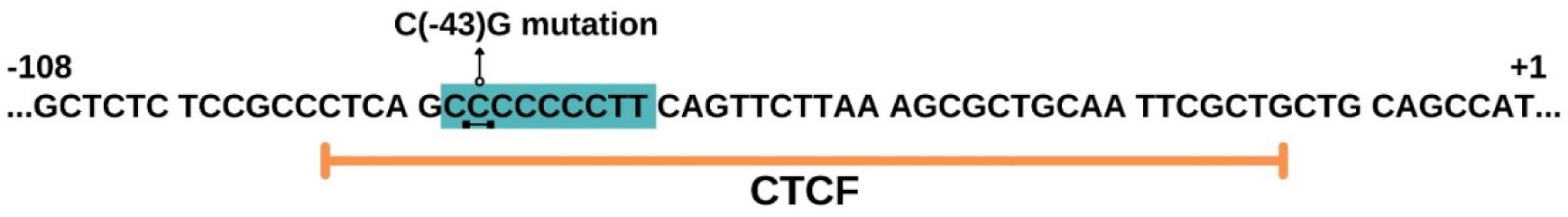
Pugacheva EM, Tiwari VK, Abdullaev Z, et al. (2005) Familial cases of point mutations in the XIST promoter reveal a correlation between CTCF binding and pre-emptive choices of X chromosome inactivation. Hum Mol Genet 14: 953-965. doi: 10.1093/hmg/ddi089
|
| [43] |
Chang SC, Brown CJ (2010) Identification of regulatory elements flanking human XIST reveals species differences. BMC Mol Biol 11: 1-10. doi: 10.1186/1471-2199-11-20
|
| [44] |
Hong Y-K, Ontiveros SD, Strauss WM (2000) A revision of the human XIST gene organization and structural comparison with mouse Xist. Mamm Genome 11: 220-224. doi: 10.1007/s003350010040
|
| [45] |
Löwdin PO (1963) Proton tunneling in DNA and its biological implications. Rev Mod Phys 35: 724. doi: 10.1103/RevModPhys.35.724
|
| [46] | Naumova AK, Plenge RM, Bird LM, et al. (1996) Heritability of X chromosome--inactivation phenotype in a large family. Am J Hum Genet 58: 1111. |
| [47] |
Newall AE, Duthie S, Formstone E, et al. (2001) Primary non-random X inactivation associated with disruption of Xist promoter regulation. Hum Mol Genet 10: 581-589. doi: 10.1093/hmg/10.6.581
|
| [48] |
Tomkins DJ, McDonald HL, Farrell SA, et al. (2002) Lack of expression of XIST from a small ring X chromosome containing the XIST locus in a girl with short stature, facial dysmorphism and developmental delay. Eur J Hum Genet 10: 44-51. doi: 10.1038/sj.ejhg.5200757
|
| [49] |
Chao W, Huynh KD, Spencer RJ, et al. (2002) CTCF, a candidate trans-acting factor for X-inactivation choice. Science 295: 345-347. doi: 10.1126/science.1065982
|
| [50] |
Donohoe ME, Zhang L-F, Xu N, et al. (2007) Identification of a Ctcf cofactor, Yy1, for the X chromosome binary switch. Mol Cell 25: 43-56. doi: 10.1016/j.molcel.2006.11.017
|
| [51] |
Sun S, Del Rosario BC, Szanto A, et al. (2013) Jpx RNA activates Xist by evicting CTCF. Cell 153: 1537-1551. doi: 10.1016/j.cell.2013.05.028
|
| [52] |
Orishchenko KE, Pavlova SV, Elisaphenko EA, et al. (2012) A regulatory potential of the Xist gene promoter in vole M. rossiaemeridionalis. PloS One 7: e33994. doi: 10.1371/journal.pone.0033994
|
| [53] |
Leontis NB, Westhof E (1998) Conserved geometrical base-pairing patterns in RNA. Q Rev Biophys 31: 399. doi: 10.1017/S0033583599003479
|
| [54] |
Leontis NB, Westhof E (2001) Geometric nomenclature and classification of RNA base pairs. Rna 7: 499-512. doi: 10.1017/S1355838201002515
|
| [55] |
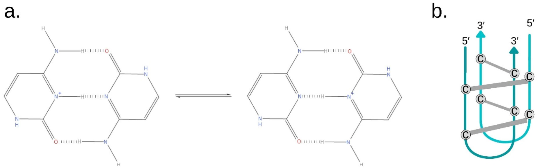
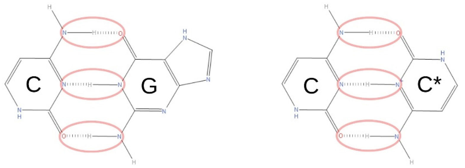
Gehring K, Leroy JL, Guéron M (1993) A tetrameric DNA structure with protonated cytosine-cytosine base pairs. Nature 363: 561-565. doi: 10.1038/363561a0
|
| [56] |
Abou Assi H, Garavís M, González C, et al. (2018) i-Motif DNA: structural features and significance to cell biology. Nucleic Acids Res 46: 8038-8056. doi: 10.1093/nar/gky735
|
| [57] |
Lieblein AL, Fürtig B, Schwalbe H (2013) Optimizing the kinetics and thermodynamics of DNA i-Motif folding. ChemBioChem 14: 1226-1230. doi: 10.1002/cbic.201300284
|
| [58] |
Benabou S, Aviñó A, Eritja R, et al. (2014) Fundamental aspects of the nucleic acid i-motif structures. Rsc Adv 4: 26956-26980. doi: 10.1039/C4RA02129K
|
| [59] |
Snoussi K, Nonin-Lecomte S, Leroy JL (2001) The RNA i-motif. J Mol Biol 309: 139-153. doi: 10.1006/jmbi.2001.4618
|
| [60] |
Dzatko S, Krafcikova M, Hänsel-Hertsch R, et al. (2018) Evaluation of the stability of DNA i-Motifs in the nuclei of living mammalian cells. Angew Chem Int Edit 57: 2165-2169. doi: 10.1002/anie.201712284
|
| [61] |
Brazier JA, Shah A, Brown GD (2012) I-motif formation in gene promoters: unusually stable formation in sequences complementary to known G-quadruplexes. Chem Commun 48: 10739-10741. doi: 10.1039/c2cc30863k
|
| [62] |
Choi J, Majima T (2011) Conformational changes of non-B DNA. Chem Soc Rev 40: 5893-5909. doi: 10.1039/c1cs15153c
|
| [63] |
Brooks TA, Kendrick S, Hurley L (2010) Making sense of G-quadruplex and i-motif functions in oncogene promoters. FEBS J 277: 3459-3469. doi: 10.1111/j.1742-4658.2010.07759.x
|
| [64] |
Manzini G, Yathindra N, Xodo L (1994) Evidence for intramolecularly folded i-DNA structures in biologically relevant CCC-repeat sequences. Nucleic Acids Res 22: 4634-4640. doi: 10.1093/nar/22.22.4634
|
| [65] |
Fojtík P, Vorlícková M (2001) The fragile X chromosome (GCC) repeat folds into a DNA tetraplex at neutral pH. Nucleic Acids Res 29: 4684-4690. doi: 10.1093/nar/29.22.4684
|
| [66] |
Srivastava R (2019) The role of proton transfer on mutations. Front Chem 7: 536. doi: 10.3389/fchem.2019.00536
|
| [67] |
Cerón-Carrasco JP, Jacquemin D (2019) i-Motif DNA structures upon electric field exposure: completing the map of induced genetic errors. Theor Chem Acc 138: 35. doi: 10.1007/s00214-019-2423-4
|
| [68] |
Bicocchi MP, Migeon BR, Pasino M, et al. (2005) Familial nonrandom inactivation linked to the X inactivation centre in heterozygotes manifesting haemophilia A. Eur J Hum Genet 13: 635-640. doi: 10.1038/sj.ejhg.5201386
|
| [69] |
González-Ramos IA, Mantilla-Capacho JM, Luna-Záizar H, et al. (2020) Genetic analysis for carrier diagnosis in hemophilia A and B in the Mexican population: 25 years of experience. Am J Med Genet C 184: 939-954. doi: 10.1002/ajmg.c.31854
|
| [70] |
Pereira LV, Zatz M (1999) Screening of the C43G mutation in the promoter region of the XIST gene in females with highly skewed X-chromosome inactivation. Am J Med Genet 87: 86-87. doi: 10.1002/(SICI)1096-8628(19991105)87:1<86::AID-AJMG19>3.0.CO;2-J
|
| [71] |
Yoon SH, Choi YM (2015) Analysis of C43G mutation in the promoter region of the XIST gene in patients with idiopathic primary ovarian insufficiency. Clin Exp Reprod Med 42: 58. doi: 10.5653/cerm.2015.42.2.58
|
| [72] |
Tegmark M (2000) Importance of quantum decoherence in brain processes. Phys Rev E 61: 4194-4206. doi: 10.1103/PhysRevE.61.4194
|
| [73] | Zurek WH (1991) From quantum to classical. Phys Today 37. |
| [74] |
Ogryzko VV (1997) A quantum-theoretical approach to the phenomenon of directed mutations in bacteria (hypothesis). Biosystems 43: 83-95. doi: 10.1016/S0303-2647(97)00030-0
|
| [75] |
Bordonaro M, Ogryzko V (2013) Quantum biology at the cellular level—Elements of the research program. Biosystems 112: 11-30. doi: 10.1016/j.biosystems.2013.02.008
|
| [76] |
McFadden J, Al-Khalili J (1999) A quantum mechanical model of adaptive mutation. Biosystems 50: 203-211. doi: 10.1016/S0303-2647(99)00004-0
|
| [77] | McFadden J (2002) Quantum Evolution WW Norton & Company. |
| [78] |
Ritz T, Wiltschko R, Hore P, et al. (2009) Magnetic compass of birds is based on a molecule with optimal directional sensitivity. Biophys J 96: 3451-3457. doi: 10.1016/j.bpj.2008.11.072
|
| [79] |
Vaziri A, Plenio MB (2010) Quantum coherence in ion channels: resonances, transport and verification. New J Phys 12: 085001. doi: 10.1088/1367-2630/12/8/085001
|
| [80] |
Basieva I, Khrennikov A, Ozawa M (2021) Quantum-like modeling in biology with open quantum systems and instruments. Biosystems 201: 104328. doi: 10.1016/j.biosystems.2020.104328
|

Figures(6)

Rodrigo Lobato. A quantum mechanical approach to random X chromosome inactivation[J]. AIMS Biophysics, 2021, 8(4): 322-336. doi: 10.3934/biophy.2021026


 DownLoad: