Citation: Théo Lebeaupin, Hafida Sellou, Gyula Timinszky, Sébastien Huet. Chromatin dynamics at DNA breaks: what, how and why?[J]. AIMS Biophysics, 2015, 2(4): 458-475. doi: 10.3934/biophy.2015.4.458
| [1] | Shu Hui Yau, Fabrice Bardy, Paul F Sowman, Jon Brock . The Magnetic Acoustic Change Complex and Mismatch Field: A Comparison of Neurophysiological Measures of Auditory Discrimination. AIMS Neuroscience, 2017, 4(1): 14-27. doi: 10.3934/Neuroscience.2017.1.14 |
| [2] | Mercedes Fernandez, Juliana Acosta, Kevin Douglass, Nikita Doshi, Jaime L. Tartar . Speaking Two Languages Enhances an Auditory but Not a Visual Neural Marker of Cognitive Inhibition. AIMS Neuroscience, 2014, 1(2): 145-157. doi: 10.3934/Neuroscience.2014.2.145 |
| [3] | Byron Bernal, Alfredo Ardila . From Hearing Sounds to Recognizing Phonemes: Primary Auditory Cortex is A Truly Perceptual Language Area. AIMS Neuroscience, 2016, 3(4): 454-473. doi: 10.3934/Neuroscience.2016.4.454 |
| [4] | Eduardo Mercado III . Relating Cortical Wave Dynamics to Learning and Remembering. AIMS Neuroscience, 2014, 1(3): 185-209. doi: 10.3934/Neuroscience.2014.3.185 |
| [5] | Matthew S. Sherwood, Jason G. Parker, Emily E. Diller, Subhashini Ganapathy, Kevin Bennett, Jeremy T. Nelson . Volitional down-regulation of the primary auditory cortex via directed attention mediated by real-time fMRI neurofeedback. AIMS Neuroscience, 2018, 5(3): 179-199. doi: 10.3934/Neuroscience.2018.3.179 |
| [6] | Charles R Larson, Donald A Robin . Sensory Processing: Advances in Understanding Structure and Function of Pitch-Shifted Auditory Feedback in Voice Control. AIMS Neuroscience, 2016, 3(1): 22-39. doi: 10.3934/Neuroscience.2016.1.22 |
| [7] | Zoha Deldar, Carlos Gevers-Montoro, Ali Khatibi, Ladan Ghazi-Saidi . The interaction between language and working memory: a systematic review of fMRI studies in the past two decades. AIMS Neuroscience, 2021, 8(1): 1-32. doi: 10.3934/Neuroscience.2021001 |
| [8] | Joan Belo, Maureen Clerc, Daniele Schön . The effect of familiarity on neural tracking of music stimuli is modulated by mind wandering. AIMS Neuroscience, 2023, 10(4): 319-331. doi: 10.3934/Neuroscience.2023025 |
| [9] | Pascale Voelker, Ashley N Parker, Phan Luu, Colin Davey, Mary K Rothbart, Michael I Posner . Increasing the amplitude of intrinsic theta in the human brain. AIMS Neuroscience, 2020, 7(4): 418-437. doi: 10.3934/Neuroscience.2020026 |
| [10] | Iliyan Ivanov, Kristin Whiteside . Dyadic Brain - A Biological Model for Deliberative Inference. AIMS Neuroscience, 2017, 4(4): 169-188. doi: 10.3934/Neuroscience.2017.4.169 |
The ability to detect and process auditory inputs plays a major role in human communication. Therefore, identification and assessment of the brain mechanisms supporting this ability is critical for understanding typical and atypical communication skills, including speech and language. Over the years, animal studies provided valuable data regarding the general structure and function of the primate auditory cortex. However, the human brain is not identical to that of any animal model, and the human auditory functioning includes aspects not present in other primates (e.g., spoken language). Therefore, studies of human auditory cortex structure and function are critically important. The main constraint is the fact that many of the effective techniques used to examine animal brains cannot be systematically applied to humans due to the invasive nature (e.g., intracranial recordings) and/or ethical concerns (e.g., experimental auditory deprivation). Advancements in non-invasive neuroimaging techniques (e.g., functional magnetic resonance imaging, fMRI; electroencephalography, EEG; magnetoencephalography, MEG; optical imaging) provide an opportunity to examine various aspects of human auditory cortex functions. These methods have yielded valuable results replicating and extending findings from the animal models.
This review focuses on the uses of scalp-recorded cortical event-related potentials (ERPs) for investigation of human auditory function. For readers interested in the evoked responses reflecting subcortical neural mechanisms of auditory processing, [1] and [2] provide relevant information. Following a brief introduction to the ERPs, the remaining sections demonstrate the success of using ERPs to address questions related to cortical maturation, functional organization, and plasticity, which have been previously studied using more invasive methods. A separate section examines studies of human auditory development and functioning following deprivation as well as restoration of auditory input. The final section describes ERP studies of multisensory interactions in the auditory cortex. From this review it should be clear that ERPs can be a valuable tool for investigating a wide range of questions concerning neural mechanisms supporting human auditory processing and provide novel insights into brain-behavior connections in the area of speech and language.
The ERP is a portion of the EEG that is time-locked to a stimulus event (see Figure 1). It reflects a momentary change in the ongoing electrical brain activity in response to an external or internal stimulus. This temporal synchronization with the evoking event allows to separate stimulus-related brain activity from the continuous background EEG when averaged across multiple trials [3]. It is important to note that the ERPs reflect oscillatory brain activity that is time- and phase-locked to stimulus onset. Examining time- but not phase-locked activity (known as the induced signal) by means of a time-frequency analysis could provide additional information about the neural mechanisms of interest (e.g., [4,5]), but is beyond the scope of this paper.
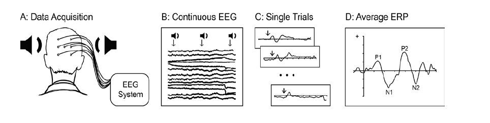 Figure 1. Schematic representation of ERP acquisition. (A). Scalp electrodes (n = 2 to 256) record electrical brain activity (electroencephalogram, EEG) while the auditory stimuli are presented repeatedly through speakers or headphones. (B). Stimulus onset/offset markers are recorded along with the continuous EEG signal. (C). Individual segments locked to stimulus onset are extracted from the continuous EEG and include a brief pre-stimulus baseline in addition to the post-stimulus period of interest. (D). Averaged ERP waveform reflects time- and phase-locked neural activity associated with stimulus processing.
ERPs waveforms are described as a series of positive and negative peaks characterized in terms of size, or amplitude (µV height of the wave at different points), latency (time from stimulus onset), scalp distribution, and more recently, brain sources of measured activity. The peaks are labeled by polarity (‘P’ for positive and ‘N’ for negative deflections) and by latency (e.g., ‘N100’ indicates a negative peak occurring at 100 ms after the stimulus event) or sequential number (‘N1’ reflects the first negative peak after stimulus onset). ERPs offer a very high temporal resolution measuring voltage changes in milliseconds and show reliable sensitivity in detecting functional changes of brain activity [6,7].
The millisecond-level resolution is the major strength of the ERPs and represents an advantage over other imaging techniques (e.g., fMRI) as it tracks information processing at the speed comparable to that of the brain processes. This is particularly important for measures of auditory function because it allows for the fine-grained level of analysis needed to accurately characterize brain’s ability to process auditory inputs, including rapidly changing speech sounds [8].
The auditory ERP studies have used a wide variety of auditory stimuli (from simple clicks and tones to syllables, words, and complex sentences) and can be broadly categorized into two types: (1) those assessing individual stimulus detection and processing and (2) those measuring differentiation of contrasting stimuli. Stimulus processing studies may include a single stimulus or multiple stimuli of interest and focus on ERP characteristics associated with the individual sounds. Conversely, auditory differentiation studies use at least two stimuli that differ on a particular dimension of interest, such as basic physical characteristics (e.g., frequency, duration), articulatory features (e.g., voice onset timing, place of articulation), or semantic aspects (e.g., real vs. nonsense words). The analyses then examine the difference in ERPs elicited by the contrasting stimuli. For a more detailed introduction to the ERP technique, including experimental design and data interpretation issues, see [9,10].
Generally, variations in ERP peaks are interpreted to reflect speed (latency) or extent (amplitude) of processing. Shorter latencies indicate more rapid processing while larger amplitudes might suggest increased brain activity (i.e., a greater number of neurons firing in synchrony). The ERP responses thought to reflect activity of the primary and secondary auditory cortex include P1, N1, P2, and mismatch negativity (MMN); however, their specific latencies and scalp distribution vary with age (see [11,12,13], for further details).
The passive nature of many ERP paradigms is an additional benefit of this technique. Behavioral measures of auditory processing typically rely on participant’s overt reaction to auditory stimulation, such as moving (e.g., turning head, raising hand, or pushing a button) or speaking. Unfortunately, the developmental level of the participant limits the use of such procedures, and the results can be confounded by inattention, poor motor control, lack of motivation, and many other variables besides the auditory processing ability. On the other hand, ERPs can be obtained without participant’s active involvement in the test because cortical brain responses to auditory stimulation are detectable even in the absence of overt behavioral reactions.
One limitation of the ERP technique is that it does not offer detailed spatial resolution needed to conclusively link the electrical activity recorded on the scalp with the specific sources within the brain. Even with high-density (e.g., 128 or 256 channels) electrode arrays, not all brain electrical activity is captured due to variations in signal strength, distance from various cortical areas to the scalp, and differences in the orientation of cortical columns generating the signal. Nevertheless, studies using convergent methodologies (e.g., ERP and fMRI, lesion studies, MEG) provided consistent results identifying most likely brain sources of the commonly observed ERP responses (see [14] for a review), and therefore allow ERP data to be interpreted with regard to the anatomical aspects of auditory processing.
A vast number of ERP studies have successfully examined a wide range of questions regarding the auditory function in humans, such as cortical maturation changes, topographic organization, and sound discrimination ability. Capitalizing on the benefits of ERP methodology, these studies were able to document auditory processing in general, and speech/language processing in particular, from the earliest developmental stages (e.g., preterm infants) and throughout the lifespan.
While the basic elements of the human auditory system are already mature at birth (e.g., the cochlea [15]), and the main cortical structures (e.g., Heschl’s gyrus, superior temporal gyrus) are in place by 37 weeks gestation [16], the auditory cortex undergoes many structural and functional changes during the first few years of life [17,18]. Although cortical layer I resembles adult structure at birth, the deep layers (lower layer III and layer IV) develop between 6 months and 5 years of age, followed by maturation of the superficial layers (upper layer III and layer II) that continues until 10-12 years [17,19].
Many of these developmental changes are reflected in the maturational time course of various ERPs. Cortical auditory responses begin to emerge as early as 25 weeks conceptional age as an ERP consisting of a negative peak followed by a positive peak [20], and an auditory change discrimination could be observed in MEG data at 27 weeks gestation [21]. Because the early negative potential is typically reduced or absent in waveforms of term infants and young children, it has been interpreted to reflect an unstimulated auditory system or the activity of non-primary auditory areas [22,23].
Precursors of all major auditory ERP peaks present at 12 months of age are evident at birth, with maturation reflected in the increase of peak amplitudes and decrease in latencies [24,25,26]. However, such changes are not uniform across the peaks and do not always follow a linear trajectory [24,27]. The time course of these developmental changes may also vary by gender [28] and by the developmental stage at birth, as infants born prematurely take longer to demonstrate auditory processing comparable to that of the infants born full-term [29].
The early positive peak (often labeled P1), typically seen even in newborns and remaining the most prominent ERP response through the early childhood [24,30], has been frequently used as an index of maturation of the thalamo-cortical auditory pathway [31,32]. This peak is thought to reflect activation of cortical layers III and IV, and consistent with their rapid maturation, P1peak latency quickly shortens with age [19].
On the other hand, the N1 peak, the most pronounced auditory ERP in adult waveforms, is not always detected in infants and young children. An auditory N1 can be recorded from 3 years of age using a slow stimulation rate (1:1.2-2.4 sec; [33,34]), but its characteristics continue to mature into adolescence and young adulthood [19,35]. This delayed emergence and protracted development of the N1 response is attributed to slower maturation of the axons in cortical layers II and upper III [19].
Animal studies have demonstrated that the auditory cortex is highly organized such that various properties of the auditory stimuli (e.g., loudness, frequency, location in space) are processed by dedicated neurons (e.g., [36,37]) arranged in spatially contiguous groups. For example, intracranial recordings in awake monkeys established that auditory stimulus intensity is processed by at least three different groups of neurons, those sensitive to a specific stimulus level, and those responding to low or to high intensities [38]. Furthermore, while some neurons showed a linear increase in firing rate with the increase in stimulus intensity, others demonstrated a nonlinear pattern of response. Human ERP studies documented that increases in sound levels were associated with increased cortical activity [39,40]. Increase in click or tone level from 0 to 40 dB SL resulted in a systematic increase of P1-N1 and N1-P2 amplitudes [41] and decrease in latencies [42], with both of these measures reaching a plateau at intensities above 50-60 dB SL. More recent evidence suggests that there may not be an asymptote level for the ERP changes in response to increased stimulus intensity, as ERP amplitudes continued to increase as tone levels shifted from 30 to 90 dB SPL when stimuli were delivered with slow presentation rate [43]. Similar shortened latency of P1, N1, and P2 peaks in response to increased loudness was reported for consonant-vowel syllables as their level increased by 0, 20, or 40 dB SL above the participants’ sound discrimination threshold needed to achieve > 95% accuracy [44]. However, under these conditions, the ERP amplitudes decreased with increased sound intensity, possibly due to reduced attentional demands for discrimination of louder stimuli.
In the stimulus frequency domain, marmoset studies demonstrated that stimulus frequency is processed in the auditory cortex by bands of neurons with a distinct spatial distribution: those tuned to low frequencies located parallel to the lateral sulcus, while high-frequency contours placed perpendicular to that sulcus [45]. Human ERP measures are also sensitive to stimulus frequency. Picton et al. [46] reported a larger N1 peak in response to low- compared to high-frequency signals. Increase in signal frequency also shortened N1 peak latency [23,47,48], see also [49] for frequency effects on N1 and MMN properties.
Development of brain source analysis procedures for ERPs allowed to take scalp data another step further and to demonstrate tonotopic organization within the auditory cortex. Using current source density mapping and spatio-temporal dipole modeling, Bertrand et al. [50] demonstrated that observed differences in N1 amplitude and peak latency in response to tones of different frequency (250, 500, 1000, 2000 and 4000 Hz) were due to changes in the orientation of the brain sources in the auditory cortex. Similar topography was reported for stimulus harmonics of complex tones [47]. There, brain sources of the N1 became more frontally oriented as spectral profiles of the stimulus harmonics increased regardless of the fundamental frequencies (i.e., pitch) of the stimuli.
Using magnetic rather than electrical signal (MEG), which is primarily sensitive to location rather than orientation of the brain source, Pantev et al. [51] demonstrated that neurons activated by higher frequencies were located deeper in the supratemporal plane (see also [52]), with the depth of the Nlm (magnetic equivalent of N1) increasing linearly with the logarithm of the stimulus frequency (500, 1000 and 4000 Hz). Although not manifested in N1 peak latency changes, possibly due to largeacoustical variation of the stimuli, similar tonotopic organization was also documented for vowels, with the maps distributed perpendicular to those for pure tones [53].
In addition to the use of ERPs to assess cortical maturation and topography, a great number of studies focused on documenting specific auditory abilities, such as sound differentiation. The mismatch negativity response (MMN) has been viewed by many as a “gold standard” ERP discrimination measure. The MMN can be evoked by any perceivable physical deviance between auditory stimuli, such as differences in duration, frequency, or intensity, as well as by more complex characteristics such as voice onset time or place of articulation of speech sounds (for reviews, see [54,55,56]).
Infant MMN studies demonstrated that even an immature auditory system is capable of carrying out complex sound discriminations. Premature infants born at 30-35 weeks gestational age are capable of discriminating vowels, suggesting that the human fetus may learn to discriminate some sounds while still in the womb [57]. In addition to vowel discrimination, full-term newborns can discriminate relatively small changes in tone frequency (e.g., 1000 vs. 1100 Hz [58,59]; 500 vs. 750Hz [60]) and in duration (60-100 ms [61]; 160 ms [62]; 200 ms [60]), and do so in a manner similar to adults as reflected in the similar time course and scalp distributions of the MMN response. Interestingly, some discrimination effects were evident even when newborns were sleeping [63]. In addition to the sound duration discrimination, a developing auditory system is also sensitive to differences in the timing between the sounds, as unexpected changes in the length of the regular inter-tone interval (500 ms vs. 1500 ms) elicited an MMN response in 10-month-old infants [64].
Sensitivity to timing differences is also relevant to speech processing. Friederici et al. [65] tested the ability of 8-week-old infants in the awake and asleep state to discriminate vowel duration in natural speech syllables /baa/ and /ba/. All infants were able to detect the longer stimulus presented infrequently among the short syllables. However, when the shorter vowel was the rare stimulus, only the awake infants produced a mismatch response. The differences in outcomes were attributed to the shorter vowel being less salient than the longer stimulus and thus requiring a certain level of alertness to be detected [65]. Using similar stimuli, Pihko et al., [66] demonstrated that the ability to detect the shorter stimulus improves with age: while only some newborns could detect the short deviant (possibly due to individual differences in sleep/wake state), by 6 months of age, all infants in their study differentiated the vowels of different length.
A separate line of research demonstrated sensitivity to temporal differences as the important aspect of categorical speech perception. Intracranial recordings from primary and secondary auditory cortex in adults reflected differences in evoked responses to syllables with the voice onset time (VOT) between 40-80 ms compared to 0-20 ms [67]. While responses to longer VOT included markers of consonant release and voicing onset, the latter was greatly reduced for short VOT stimuli. The temporal distribution of such differences matched behavioral sound discrimination data indicating a categorical shift in consonant identification from a voiced to an unvoiced stop consonant as the VOT increased from 20 to 40 ms [67]. Examining N1 amplitude in response to two-tone non-speech stimuli resembling the temporal delay of voice-onset time (VOT), Simos and Molfese [68] demonstrated that similar sensitivity to the temporal lag in sound elements is already present within 48 hours from birth. The categorical boundaries for consonant-vowel speech syllables are similar in infants, children and adults [69,70,71].
Human auditory system is also adept at discriminating other phonetic characteristics such as formant transitions associated with differences in the place of articulation (POA; [72]). Similar to the VOT findings, even young infants can discriminate consonants varying in POA (newborns—[70]; 2-4 month olds—[73], [74]). Amplitude of the P2 varies in response to POA contrasts and can be predictive of later language outcomes [75]. MMN responses in children (7-11 years) and adults are also sensitive to POA features and were present in response to synthesized speech variants of the syllable /da/ presented among standard /da/ stimuli, even though these sounds appeared to be indiscriminable using behavioral paradigms [76].
Examination of ERPs to speech sounds also highlighted hemisphere differences in auditory processing. While both VOT and POA differences affect ERPs over both hemispheres (e.g., the N1 response in adults), they also elicit lateralized ERP changes. Timing differences are more likely to be seen over the right hemisphere, while POA effects are typically observed over the left hemisphere (see [77] for a review).
Animal studies in kittens and rats have shown that repetitive exposure to stimuli with specific spectral and temporal properties (e.g., modulated tones) during early development can reorganize the primary auditory cortex (e.g., expand representation of specific frequencies [78,79,80]. ERP evidence has also demonstrated the impact of postnatal auditory stimulation on human auditory development.
While basic sound detection abilities appear to be independent of auditory experience as reflected in the absence of group differences in the P2 response to a non-speech chime, P2 responses to speech sounds in premature infants (35-38 weeks gestation) were less well developed than those of full-term newborns and 1-week old infants [81] (see also [29] and [82] for effects of extreme prematurity). Most pronounced experience-related differences were evident in the increased P2 response to their mother’s voice in 1-week-old infants compared to that of newborns, while ERPs responses to the stranger’s voice did not differ between these groups [81]. However, ERP studies in very premature infants born prior to 30 weeks gestation demonstrated that environmental auditory exposure might not be sufficient for proper auditory development [82]). Brain responses (infant P1-N2 and the mismatch response) of such infants recorded at 35 weeks postconceptual age reflected auditory change detection in pure tone stimulibut had lower amplitudes compared to those of infants born closer to term, likely due to disruptions in corticogenesis processes and/or atypical auditory stimulation associated with neonatal intensive care environment (see also [83]).
ERP findings also indicate that even a brief exposure (2.5-5 hours) to auditory stimuli can alter sound processing. Cheour [84] demonstrated that passive exposure to vowels (/i/ and /y/i/ vs. /y/) could result in improved sound discrimination in newborn infants as reflected in increased MMN response. The effects of such exposure lasted at least 24 hours and generalized to similar stimuli of different pitch. Experience-dependent plasticity is also apparent in the time course of cerebral specialization for native language processing. Cheour et al. [85] assessed sound discrimination ability in a sample of Finnish and Estonian infants using vowel targets that were present in both Finnish and Estonian languages or specific to Estonian only. At 6 months of age, stimuli from both languages elicited similar MMN responses in Finnish infants. However, at 12 months of age, MMN responses were larger for the Finnish language vowels suggesting that infants became more specialized in processing sounds of their native language. Estonian infants at 12 months did not show significant differences in MMN response to the target vowels (both were common in their language) and generated a larger MMN to the Estonian vowel than the Finnish group. Similar increases in specialization of auditory processing of the native sounds were present for consonant contrasts in American infants: at 7 months of age, infants were able to discriminate non-native contrasts but the effect disappeared by 11 months, while responsiveness to native language consonant contrasts increased over time [86]. Interestingly, ERPs data also indicate that the decline in nonnative speech perception reflects reorganization rather than loss of ability [87] as ERP responses to the nonnative contrast do not disappear but occur at later latencies or different scalp areas than those typically reflecting native sound discrimination [88,89,90].
Auditory cortex retains some plasticity beyond the first year of life as experience-related changes were observed in older children and adults. For 3-6 year old Finnish children, 2 months of attendance at a school or a daycare center where French was spoken 50-90% of the time, were sufficient to develop a MMN response for a French speech contrast [91]. In adults, auditory training to discriminate VOT differences increased amplitudes of the N1-P2 responses reflecting increased neural synchrony and heightened sensitivity to previously subtle acoustic cues [92,93].
Changes in auditory processing can also be induced in a mature system following intense and targeted exposure, both in animals [94] and humans. Reinke et al. [95] examined vowel discrimination abilities in two groups of adults during two ERP sessions (600 trials per session) separated by 1 week. During that week, one group received four training sessions on vowel identification task (1080 trials). Training resulted in a decrease of the N1 and P2 latencies. A larger P2 amplitude was observed for all participants in the post-training ERP session, but the amount of increase was greater for the trained group. In a different study, the initial ERP assessment (5400 trials) was followed by 5 daily sessions (600 trails) of consonant discrimination training [96]. At the post-training ERP session, there were no training effects on the P2 amplitude, as both trained and untrained participants exhibited a larger P2 (with slight group differences in topographic distributions). One explanation for the lack of clear training effects suggests that the two groups received a very similar number of stimulus exposures and the training sessions might have been too brief to alter ERP responses beyond the change induced by the initial exposure to the stimuli. Indeed, a significant increase in P2 was observed between the first and second halves of the pre-training ERP session, suggesting that even exposure to a speech sound without explicit training goals can alter cortical processing.
The auditory system may also lose its ability to process certain auditory cues, possibly due to decreased neural synchrony [93] and/or increased refractory time [97]. Studies in rats demonstrated that with the increasing age, the auditory cortex neurons were most likely to respond to slower-changing stimuli [98]. In humans, ERP studies noted similar patterns of slowing: in older adults with and without hearing loss N1 and P2 latencies were prolonged in response to stimuli with increased VOT durations [90,93]. Alterations in the N1 response suggest that older auditory systems are less able to time-lock to the onset of voicing when there is a gap between the onset of the consonant burst and the onset of voicing or there may be a slower recovery processes from the initial excitation response to the consonant burst before neurons are able to fire again in response to the onset of voicing [97,99]. Delayed P2 latencies suggest impairments in neural mechanisms responsible for detecting complex acoustic signals associated with speech.
Animal and human studies have demonstrated that the development of the central auditory system depends on both internal (genetic) mechanisms and external (sensory) inputs [100,101]. Atypical auditory development due to auditory deprivation (such as congenital deafness or loss of hearing early in life) provides a unique opportunity to examine the role of individual experience with sound for auditory development and the extent of cortical plasticity following restoration of auditory inputs (e.g., via hearing aides or cochlear implants) at various ages.
ERP studies in persons with hearing loss demonstrate that extended sound deprivation affects auditory development. A large negativity preceding the P1 response has been seen in congenitally deaf children and in profoundly hearing-impaired children prior to activation of cochlear implants or acquisition of hearing aids [102]. This early negativity resembled ERPs of preterm infants [103] suggesting delayed cortical maturation in the absence of auditory input.
Acquired hearing loss in adults also leads to altered cortical functioning. Moderate to severe sensorineural hearing loss was associated with prolonged N1, N2, and P3 latencies as well as reduced N2 amplitudes relative to normal hearing peers [104]. Mild to moderate sensorineural hearing loss did not result in the same increase in latencies, but was associated with reduction in the amplitude of N1 [105]. Oates et al. [106] conducted a more extensive investigation into the impact of sensorineural hearing loss on the amplitude and latencies of auditory ERPs (N1, MMN, N2, P3) in response to speech syllables. They demonstrated that as degree of hearing loss increased, latencies of ERP components were prolonged and the amplitudes were reduced or absent, with the specific ERP peak alterations dependent on stimulus intensity and the degree of hearing loss. Furthermore, changes in peak latency occurred prior to changes in amplitude. Even mild (25 to 49 dB HL) threshold elevations resulted in delayed ERPs, while the amplitude reduction was evident in participants with hearing loss of at least 60 dB HL for the 65 dB SPL stimuli and 75 dB HL for the 80 dB SPL stimuli. Additionally, although reduced amplitude and delayed peak latency of auditory ERPs were also observed in normal hearing individuals with simulated hearing loss, in the participants with sensorineural hearing loss, ERP alterations were present at better signal-to-noise ratios (i.e., for more audible sounds; [106]). Several recent studies have replicated the reported peak latency delays, but also observed an increase in the amplitudes of the auditory P2 response in adults with mild-to-moderate hearing loss, suggesting increased effortful listening and the use of compensatory information processing strategies [107,108].
Evidence from studies of cats with noise-induced hearing loss suggests that enriched auditory environment can counteract some of the detrimental cortical reorganization associated with the impaired auditory processing [109]. The use of hearing aids in humans increases the range of audible inputs and can improve morphology of cortical auditory ERPs. However, the amount of change depends on the degree of sensorineural hearing loss, the intensity of the stimuli, and is not uniform across ERP components [110]. The largest improvements associated with sound amplification occurred for individuals in the severe-to-profound hearing-impaired group. At 65 dB SPL stimulus intensity, the use of hearing aids resulted in the increased amplitudes (by 50%) and decreased latencies (by 30 ms for N1), suggesting synchronous activation of a larger pool of cortical neurons compared to the unaided condition. However, for the 80 dB SPL stimuli, amplification improved only amplitudes of the N1, possibly due to the output limiting system of the hearing aids. ERP changes associated with the use of hearing aids may be due not only to the general increase in intensity of the stimuli, but to additional alterations in sound characteristics. In a sample of normal hearing adults listening to sounds via hearing aids, increases in N1-P2 amplitudes in the aided condition were related to improvement in the signal-to-noise ratio between the stimulus and low-level environmental and/or circuit noise, as both types of auditory input were amplified by the hearing aid [43].
Cochlear implants are often used to restore auditory input in patients with hearing loss for whom hearing aids do not provide sufficient benefits. ERP evidence suggests that within 6-8 months post-implantation auditory cortex undergoes significant reorganization [111] as indicated by changes in several ERP components, and some changes in stimulus processing and discrimination can be seen within days after the initial processor fitting [112,113].As the earliest cortical ERP response elicited by auditory stimuli, P1 peak latency has been used for assessment of auditory cortex development in children with hearing impairments and cochlear implant users [23,114,115]. The presence of P1 following activation of the cochlear implants supports the assumption that the deep layers of auditory cortex may develop to some extent even in the absence of auditory stimulation [116], however that development is incomplete. ERPs elicited by brief (100-200µs) clicks or pulses in pediatric implant users were similar to those of younger controls [31]. Following activation of the implant, P1 latencies for prelingually deaf children implanted by 3.5 years of age decreased at a faster rate compared to typical development and were within normal limits after 6 months of implant use [114,117], see also [118] for a review.
Longer periods of auditory deprivation may lead to more extensive alterations in the auditory cortex [119]. Several studies suggest that cross-modal reorganization may begin around 7 years of age (e.g., [120]) and consequently limit cortical ability to process inputs from the auditory system. P1 latencies for prelingually deaf children implanted after 7 years of age showed less pronounced reduction and remained outside of the normal range even after several years of implant use [111]. The lag in P1 latency remained proportionate to the length of deafness [121].
Even greater alterations are observed for the N1 response that reflects activity of the upper layers of the auditory cortex. Unlike the deeper structures, maturation of these layers is experience-dependent and does not occur if adequate auditory stimulation was not available early in life [117]. Consequently, the N1 peak is often missing or appears immature in cochlear implant users with the history of prolonged periods of deafness during childhood [116,122]. The absence of a clear N1 response may also suggest increased likelihood of difficulties with processing speech in noise (see also [123]), because better perception of degraded speech is associated with greater maturity of the upper cortical layers [121].
N1 latencies in adults with unilateral cochlear implants are usually delayed for all auditory stimuli (e.g., tones, vowels, syllables), and N1 amplitudes are reduced for speech [124]. N1 amplitude and peak latency in implant users correlate with behavioral discrimination of speech sounds (spondee identification; [125]). Opposite of normal hearing persons, N1 amplitudes in implant users are larger for low frequency sounds and reduce with the increase in stimulus frequency [126]. These findings suggest that a prolonged period of poor high frequency stimulation common in profound deafness results in cortical reorganization favoring low frequencies. Furthermore, restoration of high frequency inputs following cochlear implantation may not be sufficient to establish typical cortical organization [126]. Over 6 months after implantation, N1 latency may shorten toward normal values, but in the prelingually deaf patients such changes are less pronounced and more variable over time. Also, a more diffuse topography was noted for N1 in cochlear implant users compared to a normal hearing person [112]. A recent longitudinal study of postlingually deaf adults demonstrated increased amplitude and decreased peak latency of the N1 response after 8 weeks of cochlear implant use [127]. However, while the N1 amplitudes became comparable to those of the normal hearing group after one year of experience with the cochlear implant, the latencies remained delayed. The magnitude of the delay was related to the duration of deafness prior to the implantation.
The degree of alteration in ERPs may be stimulus specific. In postlingually deaf adults using cochlear implants, N1-P2 latencies were delayed for frequency, syllable, and vowel contrast stimuli, N1 amplitudes were reduced for all speech stimuli, but the P2 was smaller for consonant-vowel syllables only [124]. Furthermore, ERP alterations were related to the degree of cochlear implant benefit: N1-P2 peak amplitudes and latencies in successful implant users were similar to those of normal hearing controls, and better performing users elicited larger P2 amplitudes than moderate performers [128,129]. Shorter P2 latencies were associated with shorter durations of deafness [126] and better speech perception scores [125]. Degree of benefit from the cochlear implants can also be reflected in the MMN response as its amplitude and latency are similar to those of controls in successful implant users, while in poor users, this response is typically absent [130].
Recent increase in the number of bilateral cochlear implantations further extended our understanding of the maturational processes following restoration of auditory stimulation. Infants who received bilateral cochlear implants simultaneously showed P1 latencies similar to those of age-matched hearing peers by 1 month post-activation [131]. P1 development in infants receiving two cochlear implants sequentially by 12 to 24 months of age was similar to that of unilateral cochlear implant users with latencies reaching normal limits by 3 to 6 months following the first implant acquisitions. However, after receiving the second cochlear implant, P1 latencies for that ear were within normal limits within 1 month following implantation [131]. Similar fast normalization of P1 was reported for a child receiving sequential implants prior to the age of 3.5 years [113]. In a child receiving the second implant after 7 years of age, ERPs remained similar to those observed in late-implanted unilateral implant users, suggesting that stimulation from the first implant provided minimal impact on the ipsilateral auditory cortex development [113] .
Animal studies have consistently demonstrated that the auditory cortex could be a multisensory structure, and sound processing may be affected by inputs from other modalities [132]. Parallel findings have been obtained in humans (see [133,134] for detailed reviews). Sams et al. [135] were among the first to use ERPs to demonstrate that when auditory inputs (e.g., a spoken syllable) were paired with incongruent visual stimuli (e.g., lip movements corresponding to a different syllable), the listeners tended to misidentify the auditory stimulus, and the resulting illusory percept was treated by the auditory cortex as a novel acoustic event (i.e., the McGurk effect [136]), eliciting an MMN response (see also [137,138]).
Other findings indicate that multisensory effects may be present even earlier in time as reflected in the superadditive effects where an ERP response to a multimodal stimulus is greater than the sum of the responses to its unimodal components. When the auditory, visual, and audiovisual objects were attended, the P1 (P50 in the author’s notation) to the audiovisual stimuli was larger than the sum of its amplitudes for the auditory and visual stimuli presented alone [139]. However, in the unattended condition, the P1 response to multisensory trials was smaller, similar to the sensory gating effect filtering out irrelevant inputs [140]. Giard and Peronnet [141] reported increased amplitude of the auditory N1-P2 complex in multisensory trials (tones presented simultaneously with circles). This increase exceeded the sum of the auditory and visual ERP responses. The observed multisensory effects varied among participants. For those better in visual object recognition, adding a visual cue to the auditory stimulus increased the activity in the auditory cortex. Conversely, for participants performing better in the auditory task, adding a visual cue to the auditory stimulus did not result in the change of activity in the auditory cortex. The results suggest that at an early stage of sensory analysis, multisensory integration enhanced neural activity for the nondominant modality [141]. However, a number of recent studies report evidence of such early multisensory integration effects only when auditory and visual stimuli are both attended to [139] and provide redundant information. When visual stimuli were task-irrelevant, multisensory enhancement was observed only for later ERP responses thought to reflect cognitive rather than predominantly sensory processes [142].
In addition to the superadditive response described above, ERP studies also documented the existence of a multisensory suppression phenomenon. Van Wassenhove and colleagues [143] demonstrated that audiovisual speech stimuli resulted in reduced N1-P2 responses compared to the auditory speech alone. Interestingly, amplitude reduction was independent of the audiovisual speech congruency, participants’ expectations, or attended modality. Similar evidence for suppressive, speech-specific audiovisual integration mechanisms was provided by Besle and colleagues [144,145] who reported a decrease of N1 in response to audiovisual syllables, possibly reflecting attempts to minimize the processing of redundant cross-modal information.
Visual speech also appears to speed up cortical processing of auditory signals as indicated by the reduction in the auditory N1 latency. This effect depended on visual saliency of the stimulus and was not found during object recognition [141] or discrimination of verbal material presented in spoken and written forms [146]. Given the interpretation of the auditory N1 as reflecting stimulus feature analysis [147], these findings suggest that lip movements may facilitate feature analysis of the syllables in the auditory cortex, an interpretation consistent with the behavioral evidence of faster identification of multimodal compared to auditory syllables [144,148].
The differences in the direction of the multisensory effects could be attributed to the more complex nature of the speech stimuli. However, other findings suggest that these effects are not speech-specific as the multisensory suppression occurred for both congruent and incongruent speech [148] and non-speech [149] multimodal stimuli. The more likely source of the differences is the physical arrangement of the stimuli. In most cases of audiovisual speech, the onset of the visual stimuli precedes that of the sound, while in studies showing superadditive effects, the onsets of stimuli in both modalities were simultaneous. Asynchronous stimulus onset violates the temporal congruence requirement of the superadditive responses and can reflect activity of the subcortical structures sensitive to audiovisual asynchrony [150], which in turn may lead to response suppression in the sensory specific cortices. A study by Stekelenburg and Vroomen [149] further supported and extended the role of temporal asynchrony in the generation of multisensory effects. Both N1 and P2 suppression effects were observed for speech and non-speech stimuli. However, the reduction in amplitude and peak latency of the N1 depended mainly on the presence of anticipatory motion in the visual stimulus rather than its congruence with the auditory stimuli. The N1 suppression effect did not occur in the absence of the anticipatory motion. On the other hand, the amplitude reduction of the P2 was larger for incongruent than congruent multimodal stimuli [149].
Studies focused on understanding human auditory function and its cortical mechanisms achieved great success in using measures of brain activity, such as ERPs, to address a wide range of research questions. As demonstrated in the present review, the ERP has proved to be a reliable correlate of sound detection, speech processing, and multisensory integration in the auditory cortex. The noninvasive nature and ease of acquisition of ERPs allowed researchers to compare auditory function between infants, children, and adults, track maturational changes across the lifespan, document the role of postnatal experience (or lack thereof) in auditory cortex development, and understand the contribution of auditory processing to general cognitive functioning.
Methodological advances, including the development of novel analysis techniques for modeling brain sources of scalp activity, allowed ERPs to be used not only for general detection of brain responses to sounds but for examination of more advanced questions concerning specific functional organization and plasticity of the auditory cortex previously studied using more invasive methods. Paired with new clinical developments, such as cochlear implantation that restores auditory input for persons with hearing loss, ERPs provided a unique opportunity to track cortical development and document critical periods for various auditory functions. Auditory ERP measures have also demonstrated good correspondence with the results of standardized behavioral assessments, increasing ERP utility as a potential assessment tool, especially in populations with limited behavioral repertoire (e.g., young infants) or cognitive impairments precluding them from complying with instructions and providing valid overt responses.
The next frontier for ERP applications to the study of auditory processing would be to move from their nearly exclusive use as a research tool for group-level analyses (e.g., comparing groups with and without hearing loss) to interpreting single person data in a diagnostic way, similar to the clinical use of auditory brainstem responses (ABR). ERPs are highly sensitive to developmental and individual differences. Establishment of age-specific normative criteria for ERP peak characteristics (e.g., amplitude, latency, and topographic distribution) as well as the identification of stimuli and testing paradigms with the best diagnostic value would lead to further advancements in understanding of typical and atypical auditory processes. Our improved ability to conclusively interpret individual ERPs would provide an important bridge between psychophysiological research and clinical or educational practice, leading to new developments in prevention, early detection, and effective treatment of deficits in auditory function.
This work was supported in part by NICHD grants P30HD15052 and U54 HD083211 to the Vanderbilt Kennedy Center for Research on Human Development. The figure was created by Kylie Muccilli.
The author declares no conflicts of interest in this paper.
| [1] | Woodcock CL, Ghosh RP (2010) Chromatin higher-order structure and dynamics. Cold Spring Harb Perspect Biol 2: a000596. |
| [2] |
Sexton T, Cavalli G (2015) The role of chromosome domains in shaping the functional genome. Cell 160: 1049–1059. doi: 10.1016/j.cell.2015.02.040

|
| [3] |
Miné-Hattab J, Rothstein R (2012) Increased chromosome mobility facilitates homology search during recombination. Nat Cell Biol 14: 510–517. doi: 10.1038/ncb2472
|
| [4] |
Khurana S, Kruhlak MJ, Kim J, et al. (2014) A macrohistone variant links dynamic chromatin compaction to BRCA1-dependent genome maintenance. Cell Rep 8: 1049–1062. doi: 10.1016/j.celrep.2014.07.024
|
| [5] |
Robinson PJJ, Fairall L, Huynh VAT, et al. (2006) EM measurements define the dimensions of the “30-nm” chromatin fiber: evidence for a compact, interdigitated structure. Proc Natl Acad Sci U S A 103: 6506–6511. doi: 10.1073/pnas.0601212103
|
| [6] |
Schalch T, Duda S, Sargent DF, et al. (2005) X-ray structure of a tetranucleosome and its implications for the chromatin fibre. Nature 436: 138–141. doi: 10.1038/nature03686
|
| [7] | Joti Y, Hikima T, Nishino, et al. (2012) Chromosomes without a 30-nm chromatin fiber. Nucl Austin Tex 3: 404–410. |
| [8] |
Fussner E, Ahmed K, Dehghani, et al. (2010) Changes in chromatin fiber density as a marker for pluripotency. Cold Spring Harb Symp Quant. Biol 75: 245–249. doi: 10.1101/sqb.2010.75.012
|
| [9] |
Yokota H, van den Engh G, Hearst JE, et al. (1995) Evidence for the organization of chromatin in megabase pair-sized loops arranged along a random walk path in the human G0/G1 interphase nucleus. J Cell Biol 130: 1239–1249. doi: 10.1083/jcb.130.6.1239
|
| [10] |
Petrascheck M, Escher D, Mahmoudi T et al. (2005) DNA looping induced by a transcriptional enhancer in vivo. Nucleic Acids Res. 33: 3743–3750. doi: 10.1093/nar/gki689
|
| [11] | Pombo A, Dillon N (2015) Three-dimensional genome architecture: players and mechanisms. Nat Rev Mol Cell Biol 16: 245–257. |
| [12] |
Dixon JR, Selvaraj S, Yue F, et al. (2012) Topological domains in mammalian genomes identified by analysis of chromatin interactions. Nature 485: 376–380. doi: 10.1038/nature11082
|
| [13] |
Nora EP, Lajoie BR, Schulz EG, et al. (2012) Spatial partitioning of the regulatory landscape of the X-inactivation centre. Nature 485: 381–385. doi: 10.1038/nature11049
|
| [14] |
Sexton T, Yaffe E, Kenigsberg E, et al. (2012) Three-dimensional folding and functional organization principles of the Drosophila genome. Cell 148: 458–472. doi: 10.1016/j.cell.2012.01.010
|
| [15] |
Lieberman-Aiden E, van Berkum NL, Williams L, et al. (2009) Comprehensive mapping of long-range interactions reveals folding principles of the human genome. Science 326: 289–293. doi: 10.1126/science.1181369
|
| [16] |
Bolzer A, Kreth G, Solovei I, et al. (2005) Three-dimensional maps of all chromosomes in human male fibroblast nuclei and prometaphase rosettes. PLoS Biol 3: e157. doi: 10.1371/journal.pbio.0030157
|
| [17] | Cremer T, Cremer M (2010) Chromosome territories. Cold Spring Harb Perspect Biol 2: a003889. |
| [18] | Kinney NA, Onufriev AV, Sharakhov IV (2015) Quantified effects of chromosome-nuclear envelope attachments on 3D organization of chromosomes. Nucl Austin Tex 6: 212–224. |
| [19] |
Heun P, Laroche T, Shimada K, et al. (2001) Chromosome dynamics in the yeast interphase nucleus. Science 294: 2181–2186. doi: 10.1126/science.1065366
|
| [20] |
Levi V, Ruan Q, Plutz M, et al. (2005) Chromatin dynamics in interphase cells revealed by tracking in a two-photon excitation microscope. Biophys J 89: 4275–4285. doi: 10.1529/biophysj.105.066670
|
| [21] | Hubner M, Spector D (2010) Chromatin Dynamics. Annu Rev Biophys 39: 471–489. |
| [22] | Javer A, Long Z, Nugent E, et al. (2013) Short-time movement of E. coli chromosomal loci depends on coordinate and subcellular localization. Nat Commun. 4: 3003. |
| [23] |
Gibcus JH, Dekker J (2013) The hierarchy of the 3D genome. Mol Cell 49: 773–782. doi: 10.1016/j.molcel.2013.02.011
|
| [24] |
Weber SC, Spakowitz AJ, Theriot JA (2012) Nonthermal ATP-dependent fluctuations contribute to the in vivo motion of chromosomal loci. Proc Natl Acad Sci U S A 109: 7338–7343. doi: 10.1073/pnas.1119505109
|
| [25] | Pliss A, Malyavantham KS, Bhattacharya S, et al. (2013) Chromatin dynamics in living cells: identification of oscillatory motion. J Cell Physiol 228, 609–616. |
| [26] |
Gerlich D, Beaudouin J, Kalbfuss B, et al. (2003) Global chromosome positions are transmitted through mitosis in mammalian cells. Cell 112: 751–764. doi: 10.1016/S0092-8674(03)00189-2
|
| [27] |
Walter J, Schermelleh L, Cremer M, et al. (2003) Chromosome order in HeLa cells changes during mitosis and early G1, but is stably maintained during subsequent interphase stages. J Cell Biol 160: 685–697. doi: 10.1083/jcb.200211103
|
| [28] |
Müller I, Boyle S, Singer RH, et al. (2010) Stable morphology, but dynamic internal reorganisation, of interphase human chromosomes in living cells. PloS One 5: e11560. doi: 10.1371/journal.pone.0011560
|
| [29] |
Kruhlak MJ, Celeste A, Dellaire G, et al. (2006) Changes in chromatin structure and mobility in living cells at sites of DNA double-strand breaks. J Cell Biol 172: 823–834. doi: 10.1083/jcb.200510015
|
| [30] |
Zink D, Cremer T, Saffrich R, et al. (1998) Structure and dynamics of human interphase chromosome territories in vivo. Hum Genet 102: 241–251. doi: 10.1007/s004390050686
|
| [31] |
Jackson DA, Pombo A (1998) Replicon clusters are stable units of chromosome structure: evidence that nuclear organization contributes to the efficient activation and propagation of S phase in human cells. J Cell Biol 140: 1285–1295. doi: 10.1083/jcb.140.6.1285
|
| [32] |
Robinett CC, Straight A, Li G, et al. (1996) In vivo localization of DNA sequences and visualization of large-scale chromatin organization using lac operator/repressor recognition. J Cell Biol 135: 1685–1700. doi: 10.1083/jcb.135.6.1685
|
| [33] |
Jacome A, Fernandez-Capetillo O (2011) Lac operator repeats generate a traceable fragile site in mammalian cells. EMBO Rep 12: 1032–1038. doi: 10.1038/embor.2011.158
|
| [34] |
Dubarry M, Loïodice I, Chen CL, et al. (2011) Tight protein-DNA interactions favor gene silencing. Genes Dev 25: 1365–1370. doi: 10.1101/gad.611011
|
| [35] |
Saad H, Gallardo F, Dalvai M, et al. (2014) DNA dynamics during early double-strand break processing revealed by non-intrusive imaging of living cells. PLoS Genet 10: e1004187. doi: 10.1371/journal.pgen.1004187
|
| [36] |
Chen B, Gilbert LA, Cimini BA, et al. (2013) Dynamic imaging of genomic loci in living human cells by an optimized CRISPR/Cas system. Cell 155: 1479–1491. doi: 10.1016/j.cell.2013.12.001
|
| [37] |
Miyanari Y, Ziegler-Birling C, Torres-Padilla M-E (2013) Live visualization of chromatin dynamics with fluorescent TALEs. Nat Struct Mol Biol 20: 1321–1324. doi: 10.1038/nsmb.2680
|
| [38] |
Zidovska A, Weitz DA, Mitchison TJ (2013) Micron-scale coherence in interphase chromatin dynamics. Proc Natl Acad Sci U S A 110: 15555–15560. doi: 10.1073/pnas.1220313110
|
| [39] |
Hinde E, Kong X, Yokomori K, et al. (2014) Chromatin dynamics during DNA repair revealed by pair correlation analysis of molecular flow in the nucleus. Biophys J 107: 55–65. doi: 10.1016/j.bpj.2014.05.027
|
| [40] |
Marshall WF, Straight A, Marko JF, et al. (1997) Interphase chromosomes undergo constrained diffusional motion in living cells. Curr Biol CB 7: 930–939. doi: 10.1016/S0960-9822(06)00412-X
|
| [41] |
Bornfleth H, Edelmann P, Zink D, et al. (1999) Quantitative motion analysis of subchromosomal foci in living cells using four-dimensional microscopy. Biophys J 77: 2871–2886. doi: 10.1016/S0006-3495(99)77119-5
|
| [42] | Qian H, Sheetz MP, Elson EL (1991) Single particle tracking. Analysis of diffusion and flow in two-dimensional systems. Biophys J 60: 910–921. |
| [43] |
Rosa A, Everaers R (2008) Structure and dynamics of interphase chromosomes. PLoS Comput Biol 4: e1000153. doi: 10.1371/journal.pcbi.1000153
|
| [44] | Hajjoul H, Mathon J, Ranchon H, et al. (2013) High-throughput chromatin motion tracking in living yeast reveals the flexibility of the fiber throughout the genome. Genome Res 23: 1829–1838. |
| [45] |
Havlin S, Ben-Avraham D (2002) Diffusion in disordered media. Adv Phys 51: 187–292. doi: 10.1080/00018730110116353
|
| [46] | Doi M (1996) Introduction to polymer physics Oxford University Press. |
| [47] |
Bronstein I, Israel Y, Kepten E, et al. (2009) Transient anomalous diffusion of telomeres in the nucleus of mammalian cells. Phys Rev Lett 103: 018102. doi: 10.1103/PhysRevLett.103.018102
|
| [48] |
Dion V, Kalck V, Seeber A, et al. (2013) Cohesin and the nucleolus constrain the mobility of spontaneous repair foci. EMBO Rep 14: 984–991. doi: 10.1038/embor.2013.142
|
| [49] |
Gartenberg MR, Neumann FR, Laroche T, et al. (2004) Sir-mediated repression can occur independently of chromosomal and subnuclear contexts. Cell 119: 955–967. doi: 10.1016/j.cell.2004.11.008
|
| [50] |
Hu Y, Kireev I, Plutz M, et al. (2009) Large-scale chromatin structure of inducible genes: transcription on a condensed, linear template. J Cell Biol 185: 87–100. doi: 10.1083/jcb.200809196
|
| [51] |
Neumann FR, Dion V, Gehlen LR, et al. (2012) Targeted INO80 enhances subnuclear chromatin movement and ectopic homologous recombination. Genes Dev 26: 369–383. doi: 10.1101/gad.176156.111
|
| [52] | Chuang C-H, Carpenter AE, Fuchsova B, et al. (2006) Long-range directional movement of an interphase chromosome site. Curr Biol 16: 825–831. |
| [53] | Khanna N, Hu Y, Belmont AS (2014) HSP70 transgene directed motion to nuclear speckles facilitates heat shock activation. Curr Biol 24: 1138–1144. |
| [54] | Chubb JR, Boyle S, Perry P, et al. (2002) Chromatin motion is constrained by association with nuclear compartments in human cells. Curr Biol 12: 439–445. |
| [55] |
Lucas JS, Zhang Y, Dudko OK, et al. (2014) 3D trajectories adopted by coding and regulatory DNA elements: first-passage times for genomic interactions. Cell 158: 339–352. doi: 10.1016/j.cell.2014.05.036
|
| [56] |
Daley JM, Gaines WA, Kwon Y, et al. (2014) Regulation of DNA pairing in homologous recombination. Cold Spring Harb Perspect Biol 6: a017954. doi: 10.1101/cshperspect.a017954
|
| [57] |
Lieber MR (2010) The mechanism of double-strand DNA break repair by the nonhomologous DNA end-joining pathway. Annu Rev Biochem 79: 181–211. doi: 10.1146/annurev.biochem.052308.093131
|
| [58] |
Sonoda E, Hochegger H, Saberi A, et al. (2006) Differential usage of non-homologous end-joining and homologous recombination in double strand break repair. DNA Repair 5: 1021–1029. doi: 10.1016/j.dnarep.2006.05.022
|
| [59] |
Dion V, Kalck V, Horigome C, et al. (2012) Increased mobility of double-strand breaks requires Mec1, Rad9 and the homologous recombination machinery. Nat Cell Biol 14: 502–509. doi: 10.1038/ncb2465
|
| [60] |
Seeber A, Dion V, Gasser SM (2013) Checkpoint kinases and the INO80 nucleosome remodeling complex enhance global chromatin mobility in response to DNA damage. Genes Dev 27: 1999–2008. doi: 10.1101/gad.222992.113
|
| [61] |
Lisby M, Mortensen UH, Rothstein R (2003) Colocalization of multiple DNA double-strand breaks at a single Rad52 repair centre. Nat Cell Biol 5: 572–577. doi: 10.1038/ncb997
|
| [62] |
Nagai S, Dubrana K, Tsai-Pflugfelder M, et al. (2008) Functional targeting of DNA damage to a nuclear pore-associated SUMO-dependent ubiquitin ligase. Science 322: 597–602. doi: 10.1126/science.1162790
|
| [63] | Kalocsay M, Hiller NJ, Jentsch S (2009) Chromosome-wide Rad51 spreading and SUMO-H2A.Z-dependent chromosome fixation in response to a persistent DNA double-strand break. Mol Cell 33: 335–343. |
| [64] |
Krawczyk PM, Borovski T, Stap J, et al. (2012) Chromatin mobility is increased at sites of DNA double-strand breaks. J Cell Sci 125: 2127–2133. doi: 10.1242/jcs.089847
|
| [65] |
Aten JA, Stap J, Krawczyk PM, et al. (2004) Dynamics of DNA double-strand breaks revealed by clustering of damaged chromosome domains. Science 303: 92–95. doi: 10.1126/science.1088845
|
| [66] |
Dimitrova N, Chen Y-CM, Spector DL, et al. (2008) 53BP1 promotes non-homologous end joining of telomeres by increasing chromatin mobility. Nature 456: 524–528. doi: 10.1038/nature07433
|
| [67] |
Jakob B, Splinter J, Conrad S, et al. (2011) DNA double-strand breaks in heterochromatin elicit fast repair protein recruitment, histone H2AX phosphorylation and relocation to euchromatin. Nucleic Acids Res 39: 6489–6499. doi: 10.1093/nar/gkr230
|
| [68] | Ježková L, Falk M, Falková I, et al. (2014) Function of chromatin structure and dynamics in DNA damage, repair and misrepair: γ-rays and protons in action. Appl Radiat Isot Data Instrum Methods Use Agric Ind Med 83: 128–136. |
| [69] |
Chiolo I, Minoda A, Colmenares SU, et al. (2011) Double-strand breaks in heterochromatin move outside of a dynamic HP1a domain to complete recombinational repair. Cell 144: 732–744. doi: 10.1016/j.cell.2011.02.012
|
| [70] |
Nelms BE, Maser RS, MacKay JF, et al. (1998) In situ visualization of DNA double-strand break repair in human fibroblasts. Science 280: 590–592. doi: 10.1126/science.280.5363.590
|
| [71] |
Jakob B, Splinter J, Durante M, et al. (2009) Live cell microscopy analysis of radiation-induced DNA double-strand break motion. Proc Natl Acad Sci U S A 106: 3172–3177. doi: 10.1073/pnas.0810987106
|
| [72] |
Soutoglou E, Dorn JF, Sengupta K, et al. (2007) Positional stability of single double-strand breaks in mammalian cells. Nat Cell Biol 9: 675–682. doi: 10.1038/ncb1591
|
| [73] |
Roukos V, Voss TC, Schmidt CK, et al. (2013) Spatial dynamics of chromosome translocations in living cells. Science 341: 660–664. doi: 10.1126/science.1237150
|
| [74] |
Smerdon MJ, Lieberman MW (1978) Nucleosome rearrangement in human chromatin during UV-induced DNA- reapir synthesis. Proc Natl Acad Sci U S A 75: 4238–4241. doi: 10.1073/pnas.75.9.4238
|
| [75] |
Ziv Y, Bielopolski D, Galanty Y, et al. (2006) Chromatin relaxation in response to DNA double-strand breaks is modulated by a novel ATM- and KAP-1 dependent pathway. Nat Cell Biol 8: 870–876. doi: 10.1038/ncb1446
|
| [76] |
Burgess RC, Burman B, Kruhlak MJ, et al. (2014) Activation of DNA damage response signaling by condensed chromatin. Cell Rep 9: 1703–1717. doi: 10.1016/j.celrep.2014.10.060
|
| [77] |
Smeenk G, Wiegant WW, Marteijn JA, et al. (2013) Poly(ADP-ribosyl)ation links the chromatin remodeler SMARCA5/SNF2H to RNF168-dependent DNA damage signaling. J Cell Sci 126: 889–903. doi: 10.1242/jcs.109413
|
| [78] |
Baldeyron C, Soria G, Roche D, et al. (2011) HP1alpha recruitment to DNA damage by p150CAF-1 promotes homologous recombination repair. J Cell Biol 193: 81–95. doi: 10.1083/jcb.201101030
|
| [79] |
Ayrapetov MK, Gursoy-Yuzugullu O, Xu C, et al. (2014) DNA double-strand breaks promote methylation of histone H3 on lysine 9 and transient formation of repressive chromatin. Proc Natl Acad Sci U S A 111: 9169–9174. doi: 10.1073/pnas.1403565111
|
| [80] |
Zhu L, Brangwynne CP (2015) Nuclear bodies: the emerging biophysics of nucleoplasmic phases. Curr Opin Cell Biol 34: 23–30. doi: 10.1016/j.ceb.2015.04.003
|
| [81] |
Chubb JR, Bickmore WA (2003) Considering nuclear compartmentalization in the light of nuclear dynamics. Cell 112: 403–406. doi: 10.1016/S0092-8674(03)00078-3
|
| [82] |
Lemaître C, Soutoglou E (2015) DSB (Im)mobility and DNA repair compartmentalization in mammalian cells. J Mol Biol 427: 652–658. doi: 10.1016/j.jmb.2014.11.014
|
| [83] |
Klein IA, Resch W, Jankovic M, et al. (2011) Translocation-capture sequencing reveals the extent and nature of chromosomal rearrangements in B lymphocytes. Cell 147: 95–106. doi: 10.1016/j.cell.2011.07.048
|
| [84] |
Murr R, Loizou JI, Yang Y-G, et al. (2006) Histone acetylation by Trrap-Tip60 modulates loading of repair proteins and repair of DNA double-strand breaks. Nat Cell Biol 8: 91–99. doi: 10.1038/ncb1343
|
| [85] |
Verschure PJ, van der Kraan I, Manders EMM, et al. (2003) Condensed chromatin domains in the mammalian nucleus are accessible to large macromolecules. EMBO Rep 4: 861–866. doi: 10.1038/sj.embor.embor922
|
| [86] |
Bancaud A, Huet S, Daigle N, et al. (2009) Molecular crowding affects diffusion and binding of nuclear proteins in heterochromatin and reveals the fractal organization of chromatin. EMBO J 28: 3785–3798. doi: 10.1038/emboj.2009.340
|
| [87] |
Dinant C, de Jager M, Essers J, et al. (2007) Activation of multiple DNA repair pathways by sub-nuclear damage induction methods. J Cell Sci 120: 2731–2740. doi: 10.1242/jcs.004523
|
| [88] |
Kong X, Mohanty SK, Stephens J, et al. (2009) Comparative analysis of different laser systems to study cellular responses to DNA damage in mammalian cells. Nucleic Acids Res 37: e68. doi: 10.1093/nar/gkp221
|
| [89] |
Gilbert N, Allan J (2014) Supercoiling in DNA and chromatin. Curr Opin Genet Dev 25: 15–21. doi: 10.1016/j.gde.2013.10.013
|
| [90] |
Elbel T, Langowski J (2015) The effect of DNA supercoiling on nucleosome structure and stability. J Phys Condens Matter Inst Phys J 27: 064105. doi: 10.1088/0953-8984/27/6/064105
|
| [91] |
Polo SE (2015) Reshaping chromatin after DNA damage: the choreography of histone proteins. J Mol Biol 427: 626–636. doi: 10.1016/j.jmb.2014.05.025
|
| [92] |
Downs JA, Lowndes NF, Jackson SP (2000) A role for Saccharomyces cerevisiae histone H2A in DNA repair. Nature 408: 1001–1004. doi: 10.1038/35050000
|
| [93] |
Heo K, Kim H, Choi SH, et al. (2008) FACT-mediated exchange of histone variant H2AX regulated by phosphorylation of H2AX and ADP-ribosylation of Spt16. Mol Cell 30: 86–97. doi: 10.1016/j.molcel.2008.02.029
|
| [94] | Li A, Yu Y, Lee S-C, et al. (2010) Phosphorylation of histone H2A.X by DNA-dependent protein kinase is not affected by core histone acetylation, but it alters nucleosome stability and histone H1 binding. J Biol Chem 285: 17778–17788. |
| [95] |
Golia B, Singh HR, Timinszky G (2015) Poly-ADP-ribosylation signaling during DNA damage repair. Front Biosci Landmark Ed 20: 440–457. doi: 10.2741/4318
|
| [96] |
Poirier GG, de Murcia G, Jongstra-Bilen J, et al. (1982) Poly(ADP-ribosyl)ation of polynucleosomes causes relaxation of chromatin structure. Proc Natl Acad Sci U S A 79: 3423–3427. doi: 10.1073/pnas.79.11.3423
|
| [97] | de Murcia G, Huletsky A, Lamarre D, et al. (1986) Modulation of chromatin superstructure induced by poly(ADP-ribose) synthesis and degradation. J Biol Chem 261: 7011–7017. |
| [98] | Xu Y, Ayrapetov MK, Xu C, et al. (2012) Histone H2A.Z controls a critical chromatin remodeling step required for DNA double-strand break repair. Mol Cell 48: 723–733. |
| [99] |
Clapier CR, Cairns BR (2009) The biology of chromatin remodeling complexes. Annu Rev Biochem 78: 273–304. doi: 10.1146/annurev.biochem.77.062706.153223
|
| [100] |
Cheezum MK, Walker WF, Guilford WH (2001) Quantitative comparison of algorithms for tracking single fluorescent particles. Biophys J 81: 2378–2388. doi: 10.1016/S0006-3495(01)75884-5
|
| [101] |
Wombacher R, Heidbreder M, van de Linde S, et al. (2010) Live-cell super-resolution imaging with trimethoprim conjugates. Nat Methods 7: 717–719. doi: 10.1038/nmeth.1489
|
| [102] |
Benke A, Manley S (2012) Live-cell dSTORM of cellular DNA based on direct DNA labeling. Chembiochem Eur J Chem Biol 13: 298–301. doi: 10.1002/cbic.201100679
|
| [103] |
Hihara S, Pack C-G, Kaizu K, et al. (2012) Local nucleosome dynamics facilitate chromatin accessibility in living mammalian cells. Cell Rep 2: 1645–1656. doi: 10.1016/j.celrep.2012.11.008
|
| [104] | Récamier V, Izeddin I, Bosanac L, et al. (2014) Single cell correlation fractal dimension of chromatin: a framework to interpret 3D single molecule super-resolution. Nucl Austin Tex 5: 75–84. |
| [105] |
Ricci MA, Manzo C, García-Parajo MF, et al. (2015) Chromatin fibers are formed by heterogeneous groups of nucleosomes in vivo. Cell 160: 1145–1158. doi: 10.1016/j.cell.2015.01.054
|
| [106] |
Zhang Y, Máté G, Müller P, et al. (2015) Radiation induced chromatin conformation changes analysed by fluorescent localization microscopy, statistical physics, and graph theory. PloS One 10: e0128555. doi: 10.1371/journal.pone.0128555
|
| [107] |
Llères D, James J, Swift S, et al. (2009) Quantitative analysis of chromatin compaction in living cells using FLIM-FRET. J Cell Biol 187: 481–496. doi: 10.1083/jcb.200907029
|
| [108] |
Emanuel M, Radja NH, Henriksson A, et al. (2009) The physics behind the larger scale organization of DNA in eukaryotes. Phys Biol 6: 025008. doi: 10.1088/1478-3975/6/2/025008
|
| [109] |
Rouse P (1953) A Theory of the Linear Viscoelastic Properties of Dilute Solutions of Coiling Polymers. J Chem Phys 21: 1272–1280. doi: 10.1063/1.1699180
|
| [110] |
Weber SC, Spakowitz AJ, Theriot JA (2010) Bacterial chromosomal loci move subdiffusively through a viscoelastic cytoplasm. Phys Rev Lett 104: 238102. doi: 10.1103/PhysRevLett.104.238102
|
| [111] | Metzler R, Jeon J-H, Cherstvy AG, et al. (2014) Anomalous diffusion models and their properties: non-stationarity, non-ergodicity, and ageing at the centenary of single particle tracking. Phys Chem Chem Phys 16: 24128–24164. |
| [112] | Mirny LA (2011) The fractal globule as a model of chromatin architecture in the cell. Chromosome Res Int J Mol Supramol Evol Asp Chromosome Biol 19: 37–51. |
| [113] |
Huet S, Lavelle C, Ranchon H, et al. (2014) Relevance and limitations of crowding, fractal, and polymer models to describe nuclear architecture. Int Rev Cell Mol Biol 307: 443–479. doi: 10.1016/B978-0-12-800046-5.00013-8
|
| [114] |
Barbieri M, Chotalia M, Fraser J, et al. (2012) Complexity of chromatin folding is captured by the strings and binders switch model. Proc Natl Acad Sci U S A 109: 16173–16178. doi: 10.1073/pnas.1204799109
|
| [115] |
Mateos-Langerak J, Bohn M, de Leeuw W, et al. (2009) Spatially confined folding of chromatin in the interphase nucleus. Proc Natl Acad Sci U S A 106: 3812–3817. doi: 10.1073/pnas.0809501106
|
| [116] |
Bohn M, Heermann DW (2010) Diffusion-driven looping provides a consistent framework for chromatin organization. PloS One 5: e12218. doi: 10.1371/journal.pone.0012218
|
| [117] |
Jerabek H, Heermann DW (2014) How chromatin looping and nuclear envelope attachment affect genome organization in eukaryotic cell nuclei. Int Rev Cell Mol Biol 307: 351–381. doi: 10.1016/B978-0-12-800046-5.00010-2
|
| [118] | Cook PR, Marenduzzo D (2009) Entropic organization of interphase chromosomes. J Cell Biol 186: 825–834. |
| [119] |
Bohn M, Heermann DW (2011) Repulsive forces between looping chromosomes induce entropy-driven segregation. PloS One 6: e14428. doi: 10.1371/journal.pone.0014428
|
| [120] |
Jost D, Carrivain P, Cavalli G, et al. (2014) Modeling epigenome folding: formation and dynamics of topologically associated chromatin domains. Nucleic Acids Res 42: 9553–9561. doi: 10.1093/nar/gku698
|
| [121] |
Finan K, Cook PR, Marenduzzo D (2011) Non-specific (entropic) forces as major determinants of the structure of mammalian chromosomes. Chromosome Res Int J Mol Supramol Evol Asp Chromosome Biol 19: 53–61. doi: 10.1007/s10577-010-9150-y
|
| [122] |
Zhang B, Wolynes PG (2015) Topology, structures, and energy landscapes of human chromosomes. Proc Natl. Acad Sci U S A 112: 6062–6067. doi: 10.1073/pnas.1506257112
|
| 1. | Catherine Morgan, Linda Fetters, Lars Adde, Nadia Badawi, Ada Bancale, Roslyn N. Boyd, Olena Chorna, Giovanni Cioni, Diane L. Damiano, Johanna Darrah, Linda S. de Vries, Stacey Dusing, Christa Einspieler, Ann-Christin Eliasson, Donna Ferriero, Darcy Fehlings, Hans Forssberg, Andrew M. Gordon, Susan Greaves, Andrea Guzzetta, Mijna Hadders-Algra, Regina Harbourne, Petra Karlsson, Lena Krumlinde-Sundholm, Beatrice Latal, Alison Loughran-Fowlds, Catherine Mak, Nathalie Maitre, Sarah McIntyre, Cristina Mei, Angela Morgan, Angelina Kakooza-Mwesige, Domenico M. Romeo, Katherine Sanchez, Alicia Spittle, Roberta Shepherd, Marelle Thornton, Jane Valentine, Roslyn Ward, Koa Whittingham, Alieh Zamany, Iona Novak, Early Intervention for Children Aged 0 to 2 Years With or at High Risk of Cerebral Palsy, 2021, 175, 2168-6203, 846, 10.1001/jamapediatrics.2021.0878 |
Figures(3)

Théo Lebeaupin, Hafida Sellou, Gyula Timinszky, Sébastien Huet. Chromatin dynamics at DNA breaks: what, how and why?[J]. AIMS Biophysics, 2015, 2(4): 458-475. doi: 10.3934/biophy.2015.4.458


 DownLoad: