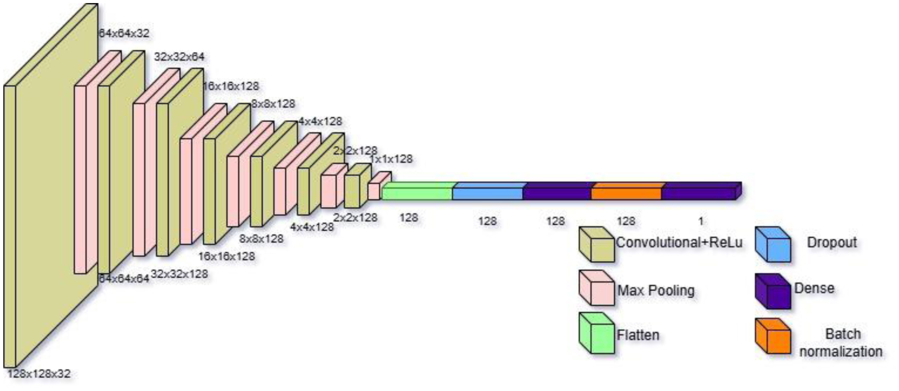
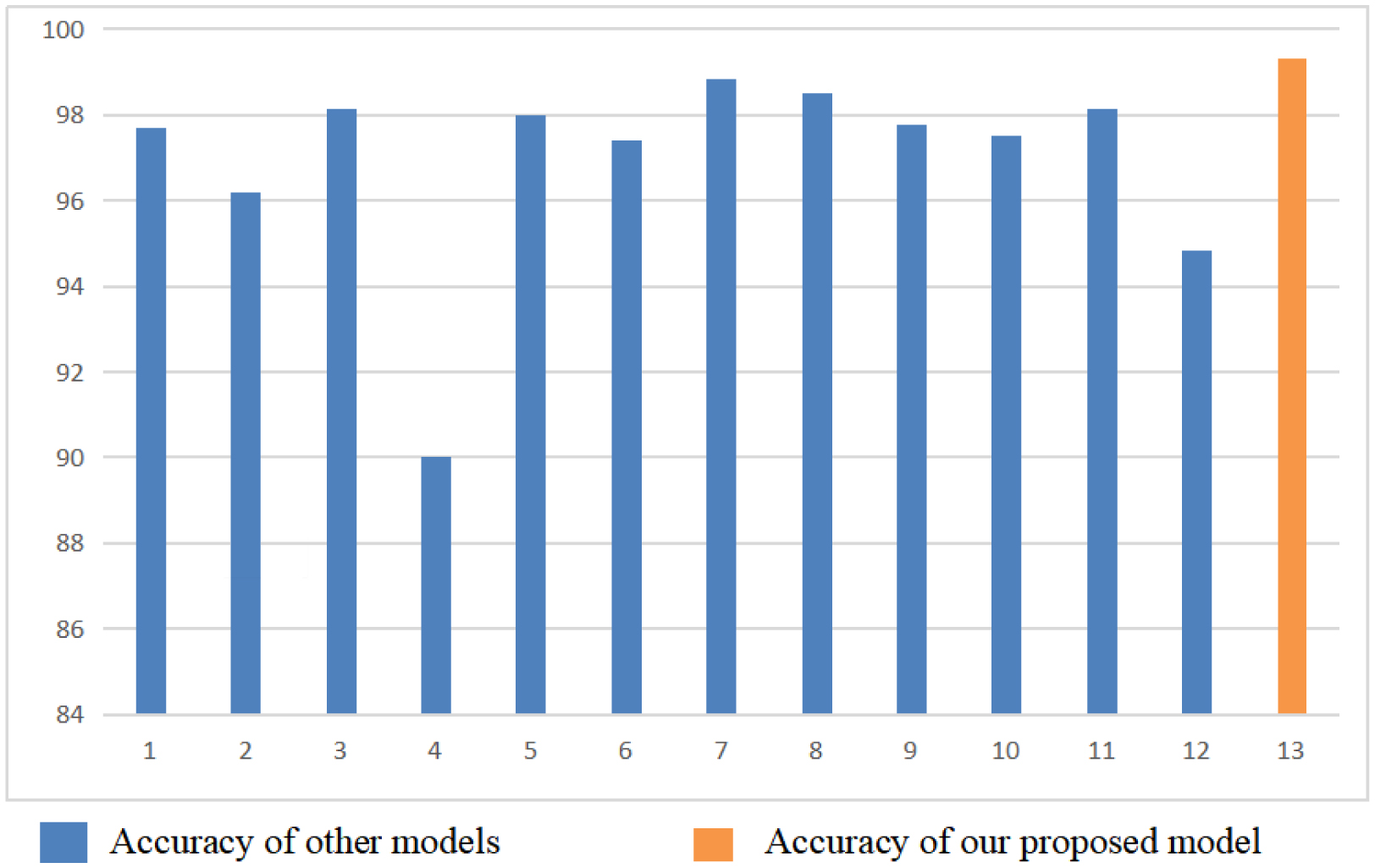
The brain is one of the most important organs of a human body. It controls all activities of the body and hence is referred to as the CPU of human body. Fast, accurate and early diagnosis of brain tumors is essential for better treatment plans that potentially result in larger survival rates. Automatic and non-invasive brain tumor detection methods are highly relevant. Continuous efforts by researchers have resulted in a significant increase in brain tumor detection accuracy, but 100% accuracy on testing/validation data is still challenging to obtain. This paper presents a convolutional neural network model that significantly enhances brain tumor classification accuracy with low complexity. To do so, Kaggle's publicly available dataset titled “Brain_Tumor_Detection_MRI”, consisting of 2891 brain MRI images annotated as “yes” (having tumors) or “no” (without tumors), was used. By leveraging advanced deep learning techniques, we achieved an accuracy of 99.31% on the test dataset. This value shows a significant improvement in classification accuracy, showcasing the potential of convolutional neural networks in medical imaging and diagnostic applications.
Citation: Abhimanu Singh, Smita Jain. Enhanced brain tumor detection from brain MRI images using convolutional neural networks[J]. AIMS Bioengineering, 2025, 12(2): 215-224. doi: 10.3934/bioeng.2025010
The brain is one of the most important organs of a human body. It controls all activities of the body and hence is referred to as the CPU of human body. Fast, accurate and early diagnosis of brain tumors is essential for better treatment plans that potentially result in larger survival rates. Automatic and non-invasive brain tumor detection methods are highly relevant. Continuous efforts by researchers have resulted in a significant increase in brain tumor detection accuracy, but 100% accuracy on testing/validation data is still challenging to obtain. This paper presents a convolutional neural network model that significantly enhances brain tumor classification accuracy with low complexity. To do so, Kaggle's publicly available dataset titled “Brain_Tumor_Detection_MRI”, consisting of 2891 brain MRI images annotated as “yes” (having tumors) or “no” (without tumors), was used. By leveraging advanced deep learning techniques, we achieved an accuracy of 99.31% on the test dataset. This value shows a significant improvement in classification accuracy, showcasing the potential of convolutional neural networks in medical imaging and diagnostic applications.

| [1] |
Singh A, Jain S (2023) Study on Variation of Prediction Accuracy of a Convolutional Neural Network Model for Brain Tumor Detection using MR Images. Proceedings of Fourth Doctoral Symposium on Computational Intelligence, DoSCI 2023. Lecture Notes in Networks and Systems . Singapore: Springer Nature 415-424. https://doi.org/10.1007/978-981-99-3716-5_35 
|
| [2] |
Seoni S, Shahini A, Meiburger KM, et al. (2020) All you need is data preparation: A systematic review image harmonization techniques in Multi-center/device studies for medical support systems. Comput Meth Prog Biomed 250: 108200. https://doi.org/10.1016/j.cmpb.2024.108200
|
| [3] |
Sun M, Song Z, Jiang X, et al. (2017) Learning pooling for convolutional neural network. Neurocomputing 224: 96-104. https://doi.org/10.1016/j.neucom.2016.10.049
|
| [4] |
Zafar A, Aamir M, Mohd Nawi N, et al. (2022) A comparison of pooling methods for convolutional neural networks. Appl Sci 12: 8643. https://doi.org/10.3390/app12178643
|
| [5] |
Abuqaddom I, Mahafzah BA, Faris H (2021) Oriented stochastic loss descent algorithm to train very deep multi-layer neural networks without vanishing gradients. Knowl-Based Syst 230: 107391. https://doi.org/10.1016/j.knosys.2021.107391
|
| [6] |
Sabri N, Hamed HNA, Ibrahim Z, et al. (2020) A comparison between average and max-pooling in convolutional neural network for scoliosis classification. Int J Adv Trends Comput Sci Eng 9: 689-696. https://doi.org/10.30534/ijatcse/2020/9791.42020
|
| [7] |
Akter A, Nosheen N, Ahmad S, et al. (2024) Robust clinical applicable CNN and U-Net based algorithm for MRI classification and segmentation for brain tumor. Expert Syst Appl 23: 122347. https://doi.org/10.1016/j.eswa.2023.122347
|
| [8] |
Ramakrishnan AB, Sridevi M, Vasudevan SK, et al. (2024) Optimizing brain tumor classification with hybrid CNN architecture: Balancing accuracy and efficiency through one API optimization. Inf Med Unlock 44: 101436. https://doi.org/10.1016/j.imu.2023.101436
|
| [9] | Deshpande A, Estrela VV, Patvardhan P (2021) The DCT-CNN-ResNet50 architecture to classify brain tumors with super-resolution, convolutional neural network, and the ResNet50. Neurosci Inf 1: 100013. https://doi.org/10.1016/j.neuri.2021.100013 |
| [10] | Gupta BB, Gaurav A, Arya V (2024) Deep CNN based brain tumor detection in intelligent systems. Int J Intell Net 5: 30-37. https://doi.org/10.1016/j.ijin.2023.12.001 |
| [11] | Rai HM, Chatterjee K (2020) Detection of brain abnormality by a novel Lu-Net deep neural CNN model from MR images. Mach Learn Appl 2: 100004. https://doi.org/10.1016/j.mlwa.2020.100004 |
| [12] |
Islam MN, Azam MS, Md Islam S, et al. (2024) An improved deep learning-based hybrid model with ensemble techniques for brain tumor detection from MRI image. Inf Med Unlock 47: 101483. https://doi.org/10.1016/j.imu.2024.101483
|
| [13] |
Al-Jammas MH, Al-Sabawi E A, Yassin A M, et al. (2024) Brain tumors recognition based on deep learning. e-Prime-Adv Electr Eng Electron Energy 8: 100500. https://doi.org/10.1016/j.prime.2024.100500
|
| [14] |
Khairandish MO, Sharma M, Jain V, et al. (2022) A hybrid CNN-SVM threshold segmentation approach for tumor detection and classification of MRI brain images. Irbm 43: 290-299. https://doi.org/10.1016/j.irbm.2021.06.003
|
| [15] |
Patil S, Kirange D (2023) Ensemble of deep learning models for brain tumor detection. Procedia Comput Sci 218: 2468-2479. https://doi.org/10.1016/j.procs.2023.01.222
|
| [16] | Shanthi S, Saradha S, Smitha JA, et al. (2022) An efficient automatic brain tumor classification using optimized hybrid deep neural network. Int J Intell Net 3: 188-196. https://doi.org/10.1016/j.ijin.2022.11.003 |
| [17] |
Rahman T, Islam Md S (2023) MRI brain tumor detection and classification using parallel deep convolutional neural networks. Measurement: Sensors 26: 100694. https://doi.org/10.1016/j.measen.2023.100694
|
| [18] |
Swati ZNK, Zhao Q, Kabir M, et al. (2019) Brain tumor classification for MR images using transfer learning and fine-tuning. Comput Med Imag Grap 75: 34-46. https://doi.org/10.1016/j.compmedimag.2019.05.001
|
| [19] |
Agrawal T, Chaudhary P, Kumar V, et al. (2024) A comparative study of brain tumor classification on unbalanced dataset using deep neural networks. Biomed Signal Proces 94: 106256. https://doi.org/10.1016/j.bspc.2024.106256
|
| [20] | Shivahare BD, Gupta SK, Katiyar AN, et al. (2023) Medical image denoising and brain tumor detection using CNN and U-Net. 3rd International Conference on Innovative Sustainable Computational Technologies (CISCT) . IEEE 1-5. https://doi.org/10.1109/CISCT57197.2023.10351338 |
| [21] |
Gursoy E, Kaya Y (2024) Brain-gcn-net: Graph-convolutional neural network for brain tumor identification. Comput Biol Med 180: 108971. https://doi.org/10.1016/j.compbiomed.2024.108971
|
Figures(4) / Tables(1)

Abhimanu Singh, Smita Jain. Enhanced brain tumor detection from brain MRI images using convolutional neural networks[J]. AIMS Bioengineering, 2025, 12(2): 215-224. doi: 10.3934/bioeng.2025010


 DownLoad: