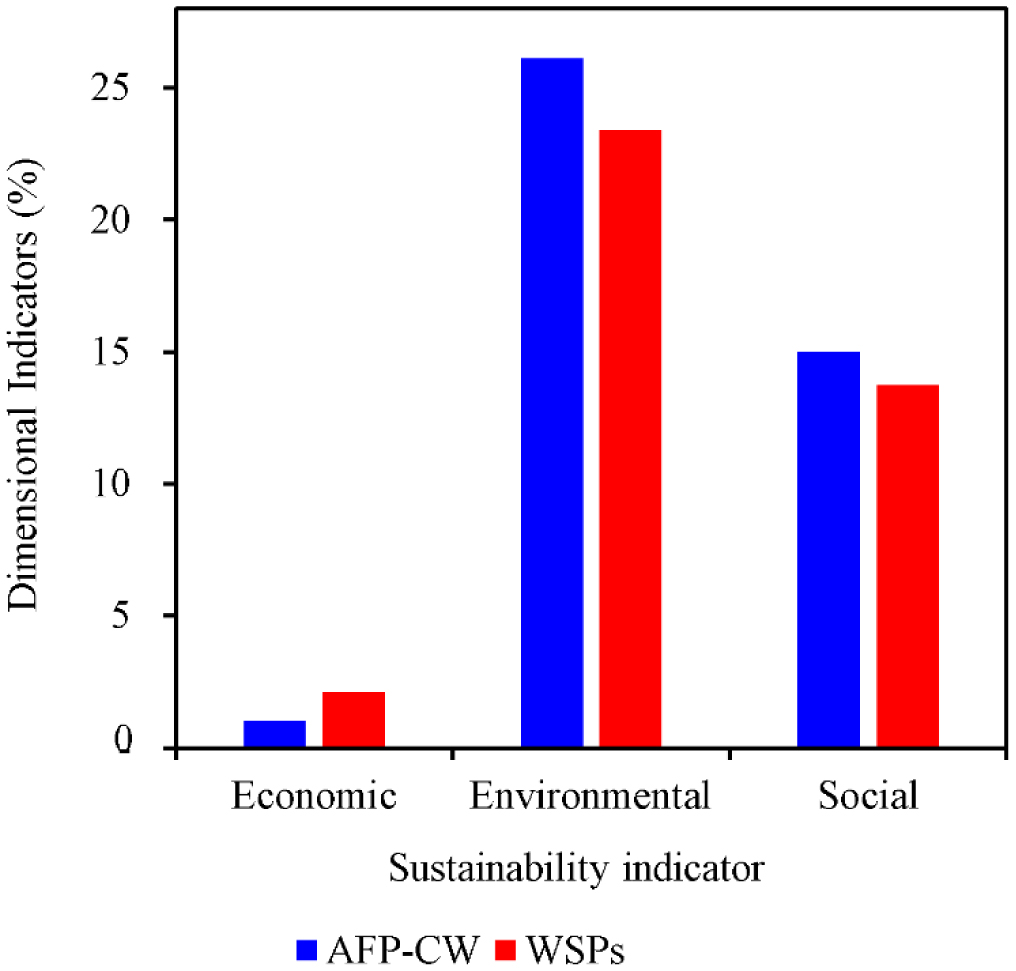
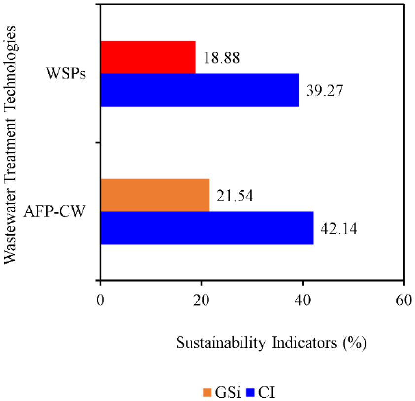
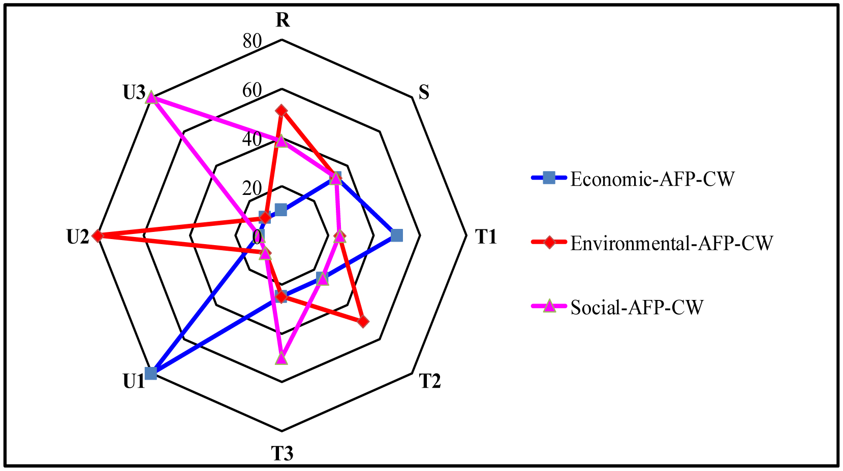
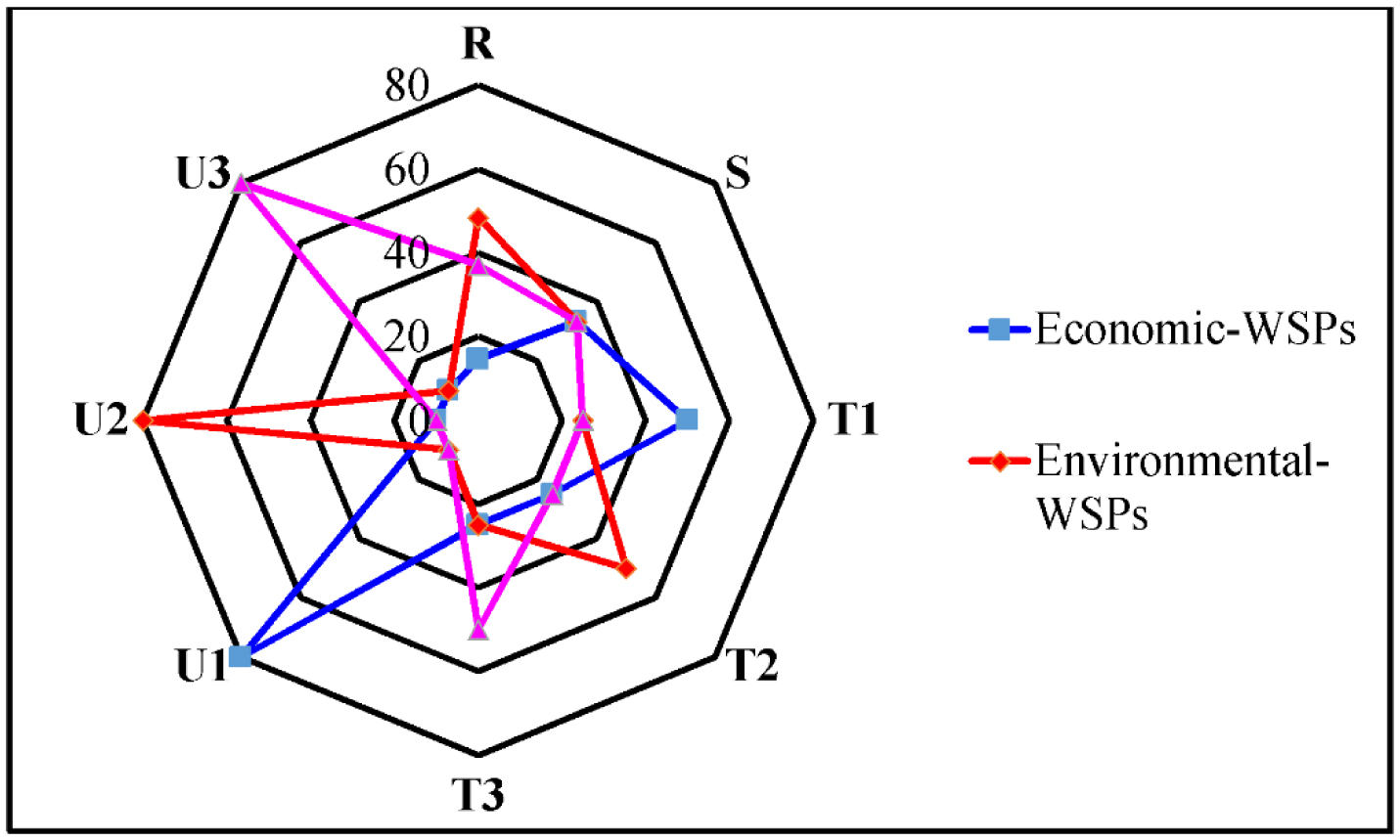
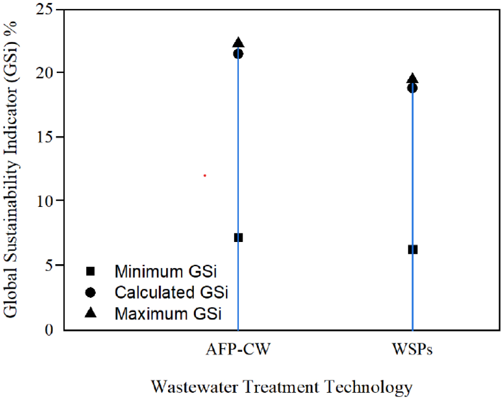
A comparative study was conducted to compare the performance of waste stabilization ponds (WSPs) with an upflow operation type advanced facultative pond integrated with constructed wetland (AFP-CW) technologies. Our aim was to address gaps in economic, environmental, and social aspects identified in traditional WSPs. Economic, environmental, and social sustainability indicators were used in a mathematical model to select a sustainable technology for organic-rich wastewater treatment for resource recovery. The results showed that for the AFP-CW, economic, environmental, and social indicators were weighted at 10.18%, 51.11%, and 38.71%, respectively, while for WSPs, the percentages were 14.55, 48.39, and 37.06, respectively. The composite sustainability indicator (CSI) for AFP-CW was 42.14% and for WSPs was 39.27%, with the global sustainability indicator (GSi) reaching 21.54% for AFP-CW and 18.88% for WSPs. A sensitivity analysis revealed that the maximum global sustainability indicator was 22.34% for AFP-CW and 19.54% for WSPs. Overall, the AFP-CW was considered a more sustainable technology for wastewater treatment, with lower economic but higher environmental and social sustainability indicators compared to WSPs, which showed higher economic but lower environmental and social sustainability indicators. The sustainability of AFP-CW is supported by its small construction area, nutrient recovery in sludge, biogas recovery, reduced global warming impact, as well as nutrient and water recycling for irrigation.
Citation: Chrisogoni Paschal, Mwemezi J. Rwiza, Karoli N. Njau. Application of sustainability indicators for the evaluation and selection of robust organic-rich wastewater treatment technology for resource recovery[J]. AIMS Bioengineering, 2024, 11(3): 439-477. doi: 10.3934/bioeng.2024020
A comparative study was conducted to compare the performance of waste stabilization ponds (WSPs) with an upflow operation type advanced facultative pond integrated with constructed wetland (AFP-CW) technologies. Our aim was to address gaps in economic, environmental, and social aspects identified in traditional WSPs. Economic, environmental, and social sustainability indicators were used in a mathematical model to select a sustainable technology for organic-rich wastewater treatment for resource recovery. The results showed that for the AFP-CW, economic, environmental, and social indicators were weighted at 10.18%, 51.11%, and 38.71%, respectively, while for WSPs, the percentages were 14.55, 48.39, and 37.06, respectively. The composite sustainability indicator (CSI) for AFP-CW was 42.14% and for WSPs was 39.27%, with the global sustainability indicator (GSi) reaching 21.54% for AFP-CW and 18.88% for WSPs. A sensitivity analysis revealed that the maximum global sustainability indicator was 22.34% for AFP-CW and 19.54% for WSPs. Overall, the AFP-CW was considered a more sustainable technology for wastewater treatment, with lower economic but higher environmental and social sustainability indicators compared to WSPs, which showed higher economic but lower environmental and social sustainability indicators. The sustainability of AFP-CW is supported by its small construction area, nutrient recovery in sludge, biogas recovery, reduced global warming impact, as well as nutrient and water recycling for irrigation.

| [1] | Obaideen K, Shehata N, Sayed ET, et al. (2022) The role of wastewater treatment in achieving sustainable development goals (SDGs) and sustainability guideline. Energy Nexus 7: 100112. https://doi.org/10.1016/j.nexus.2022.100112 |
| [2] | Schellenberg T, Subramanian V, Ganeshan G, et al. (2020) Wastewater discharge standards in the evolving context of urban sustainability—The case of India. Front Environ Sci 8: 30. https://doi.org/10.3389/fenvs.2020.00030 |
| [3] | Adamopoulos I, Syrou N, Adamopoulou J (2024) Greece's current water and wastewater regulations and the risks they pose to environmental hygiene and public health, as recommended by the European Union Commission. Eur J Sustain Dev Res 8. https://doi.org/10.29333/ejosdr/14301 |
| [4] | Sangamnere R, Misra T, Bherwani H, et al. (2023) A critical review of conventional and emerging wastewater treatment technologies. Sustain Water Resour Manag 9: 58. https://doi.org/10.1007/s40899-023-00829-y |
| [5] | Liew WL, Kassim MA, Muda K, et al. (2015) Conventional methods and emerging wastewater polishing technologies for palm oil mill effluent treatment: A review. J Environ Manage 149: 222-235. https://doi.org/10.1016/j.jenvman.2014.10.016 |
| [6] | Younas F, Mustafa A, Farooqi ZUR, et al. (2021) Current and emerging adsorbent technologies for wastewater treatment: Trends, limitations, and environmental implications. Water 13: 215. https://doi.org/10.3390/w13020215 |
| [7] | Hanafi MF, Sapawe N (2020) A review on the current techniques and technologies of organic pollutants removal from water/wastewater. Mater Today Proc 31: A158-A165. https://doi.org/10.1016/j.matpr.2021.01.265 |
| [8] | Weerakoon W, Jayathilaka N, Seneviratne KN (2023) Water quality and wastewater treatment for human health and environmental safety. Metagenomics to Bioremediation . India: Elsevier 357-378. https://doi.org/10.1016/B978-0-323-96113-4.00031-7 |
| [9] | Capodaglio A, Callegari A (2016) Domestic wastewater treatment with a decentralized, simple technology biomass concentrator reactor. J Water Sanit Hyg Dev 6: 507-510. https://doi.org/10.2166/washdev.2016.042 |
| [10] | Koul B, Yadav D, Singh S, et al. (2022) Insights into the domestic wastewater treatment (DWWT) regimes: A review. Water 14: 3542. https://doi.org/10.3390/w14213542 |
| [11] | Shrivastava P (2018) Environmental technologies and competitive advantage. Business Ethics and Strategy . New York: Routledge 317-334. https://doi.org/10.4324/9781315261102 |
| [12] | Salamirad A, Kheybari S, Ishizaka A, et al. (2023) Wastewater treatment technology selection using a hybrid multicriteria decision-making method. Int J Oper Res 30: 1479-1504. https://doi.org/10.1111/itor.12979 |
| [13] | Li J, Liu J, Yu H, et al. (2022) Sources, fates and treatment strategies of typical viruses in urban sewage collection/treatment systems: A review. Desalination 534: 115798. https://doi.org/10.1016/j.desal.2022.115798 |
| [14] | Xie Y, Zhang Q, Li Y, et al. (2023) A new paradigm of sewage collection in rural areas. Environ Sci Pollut R 30: 28609-28620. https://doi.org/10.1007/s11356-022-24014-4 |
| [15] | Withers PJ, Jordan P, May L, et al. (2014) Do septic tank systems pose a hidden threat to water quality?. Front Ecol Environ 12: 123-130. https://doi.org/10.1890/130131 |
| [16] | Gunady M, Shishkina N, Tan H, et al. (2015) A review of on-site wastewater treatment systems in Western Australia from 1997 to 2011. J Environ Public Health 2015: 12. https://doi.org/10.1155/2015/716957 |
| [17] | Wang M, Zhu J, Mao X (2021) Removal of pathogens in onsite wastewater treatment systems: A review of design considerations and influencing factors. Water 13: 1190. https://doi.org/10.3390/w13091190 |
| [18] | Nasr FA, Mikhaeil B (2015) Treatment of domestic wastewater using modified septic tank. Desalin Water Treat 56: 2073-2081. https://doi.org/10.1080/19443994.2014.961174 |
| [19] | Lusk MG, Toor GS, Yang YY, et al. (2017) A review of the fate and transport of nitrogen, phosphorus, pathogens, and trace organic chemicals in septic systems. Crit Rev Environ Sci Technol 47: 455-541. https://doi.org/10.1080/10643389.2017.1327787 |
| [20] | Abbassi B, Abuharb R, Ammary B, et al. (2018) Modified septic tank: Innovative onsite wastewater treatment system. Water 10: 578. https://doi.org/10.3390/w10050578 |
| [21] | Anil R, Neera AL (2016) Modified septic tank treatment system. Proc Technol 24: 240-247. https://doi.org/10.1016/j.protcy.2016.05.032 |
| [22] | Keshtgar L, Rostami A, Azimi AA, et al. (2019) The impact of barrier walls (baffle) on performance of septic tanks in domestic wastewater treatment. Desalin Water Treat 161: 254-259. https://doi.org/10.5004/dwt.2019.24303 |
| [23] | Yang YY, Toor GS, Wilson PC, et al. (2017) Micropollutants in groundwater from septic systems: Transformations, transport mechanisms, and human health risk assessment. Water Res 123: 258-267. https://doi.org/10.1016/j.watres.2017.06.054 |
| [24] | Kihila JM, Balengayabo JG (2020) Adaptable improved onsite wastewater treatment systems for urban settlements in developing countries. Cogent Environ Sci 6: 1823633. https://doi.org/10.1080/23311843.2020.1823633 |
| [25] | Devitt C, O'Neill E, Waldron R (2016) Drivers and barriers among householders to managing domestic wastewater treatment systems in the Republic of Ireland; implications for risk prevention behaviour. J Hydrol 535: 534-546. https://doi.org/10.1016/j.jhydrol.2016.02.015 |
| [26] | Gupta S, Mittal Y, Panja R, et al. (2021) Conventional wastewater treatment technologies. Curr Dev Biotechnol Bioeng 47–75. https://doi.org/10.1016/B978-0-12-821009-3.00012-9 |
| [27] | Ahammad SZ, Graham DW, Dolfing J (2020) Wastewater treatment: Biological. Managing Water Resources and Hydrological Systems . Boca Raton: CRC Press 561-576. https://doi.org/10.1201/9781003045045 |
| [28] | Anekwe IMS, Adedeji J, Akpasi SO, et al. (2022) Available technologies for wastewater treatment. Wastewater Treatment . London: IntechOpen. https://doi.org/10.5772/intechopen.103661 |
| [29] | Pereira CP, Barbosa AA, Bassin JP (2022) Sewage treatment through anaerobic processes: Performance, technologies, and future developments. Anaerobic Biodigesters for Human Waste Treatment . Berlin: Springer 3-28. https://doi.org/10.1007/978-981-19-4921-0_1 |
| [30] | Verma S, Kuila A, Jacob S (2023) Role of biofilms in waste water treatment. Appl Biochem Biotechnol 195: 5618-5642. https://doi.org/10.1007/s12010-022-04163-5 |
| [31] | Zhao Y, Liu D, Huang W, et al. (2019) Insights into biofilm carriers for biological wastewater treatment processes: Current state-of-the-art, challenges, and opportunities. Bioresour Technol 288: 121619. https://doi.org/10.1016/j.biortech.2019.121619 |
| [32] | Kesaano M, Sims RC (2014) Algal biofilm based technology for wastewater treatment. Algal Res 5: 231-240. https://doi.org/10.1016/j.algal.2014.02.003 |
| [33] | Pandit J, Sharma AK (2024) Advanced techniques in wastewater treatment: A comprehensive review. Asian J Environ Ecol 23: 1-26. https://doi.org/10.9734/ajee/2024/v23i10605 |
| [34] | Butler E, Hung YT, Suleiman Al Ahmad M, et al. (2017) Oxidation pond for municipal wastewater treatment. Appl Water Sci 7: 31-51. https://doi.org/10.1007/s13201-015-0285-z |
| [35] | Kamble SJ, Singh A, Kharat MG (2017) A hybrid life cycle assessment based fuzzy multi-criteria decision making approach for evaluation and selection of an appropriate municipal wastewater treatment technology. Euro-Mediterr J Envi 2: 1-17. https://doi.org/10.1007/s41207-017-0019-8 |
| [36] | Bhojwani S, Topolski K, Mukherjee R, et al. (2019) Technology review and data analysis for cost assessment of water treatment systems. Sci Total Environ 651: 2749-2761. https://doi.org/10.1016/j.scitotenv.2018.09.363 |
| [37] | Wang XH, Wang X, Huppes G, et al. (2015) Environmental implications of increasingly stringent sewage discharge standards in municipal wastewater treatment plants: Case study of a cool area of China. J Clean Prod 94: 278-283. https://doi.org/10.1016/j.jclepro.2015.02.007 |
| [38] | Castillo A, Porro J, Garrido-Baserba M, et al. (2016) Validation of a decision support tool for wastewater treatment selection. J Environ Manage 184: 409-418. https://doi.org/10.1016/j.jenvman.2016.09.087 |
| [39] | Plakas K, Georgiadis A, Karabelas A (2016) Sustainability assessment of tertiary wastewater treatment technologies: A multi-criteria analysis. Water Sci Technol 73: 1532-1540. https://doi.org/10.2166/wst.2015.630 |
| [40] | Voulvoulis N, Burgman MA (2019) The contrasting roles of science and technology in environmental challenges. Crit Rev Environ Sci Technol 49: 1079-1106. https://doi.org/10.1080/10643389.2019.1565519 |
| [41] | Irene T, Yohana L, Senzia M, et al. (2014) Modeling of municipal wastewater treatment in a system consisting of waste stabilization ponds, constructed wetlands and fish ponds in Tanzania. Developments in Environmental Modelling . Amsterdam: Elsevier 585-600. https://doi.org/10.1016/B978-0-444-63249-4.00025-7 |
| [42] | Wang H, Wang T, Zhang B, et al. (2014) Water and wastewater treatment in Africa–current practices and challenges. Clean-Soil Air Water 42: 1029-1035. https://doi.org/10.1002/clen.201300208 |
| [43] | Kihila J, Mtei KM, Njau KN (2014) Wastewater treatment for reuse in urban agriculture; the case of Moshi Municipality, Tanzania. Phys Chem Earth 72: 104-110. https://doi.org/10.1016/j.pce.2014.10.004 |
| [44] | Coggins LX, Crosbie ND, Ghadouani A (2019) The small, the big, and the beautiful: Emerging challenges and opportunities for waste stabilization ponds in Australia. Wiley Interdiscip Rev: Water 6: e1383. https://doi.org/10.1002/wat2.1383 |
| [45] | Ho LT, Van Echelpoel W, Goethals PL (2017) Design of waste stabilization pond systems: A review. Water Res 123: 236-248. https://doi.org/10.1016/j.watres.2017.06.071 |
| [46] | Bansah KJ, Suglo RS (2016) Sewage treatment by waste stabilization pond systems. J Energ Nat Res Mag 3. https://doi.org/10.26796/jenrm.v3i1.82 |
| [47] | Ho L, Goethals PL (2020) Municipal wastewater treatment with pond technology: Historical review and future outlook. Ecol Eng 148: 105791. https://doi.org/10.1016/j.ecoleng.2020.105791 |
| [48] | Adhikari K, Fedler CB (2020) Water sustainability using pond-in-pond wastewater treatment system: Case studies. J Water Process Eng 36: 101281. https://doi.org/10.1016/j.jwpe.2020.101281 |
| [49] | Adhikari K, Fedler CB (2020) Pond-In-Pond: An alternative system for wastewater treatment for reuse. J Environ Chem Eng 8: 103523. https://doi.org/10.1016/j.jece.2019.103523 |
| [50] | Tran HT, Lesage G, Lin C, et al. (2022) Activated sludge processes and recent advances. Curr Dev Biotechnol Bioeng 49–79. https://doi.org/10.1016/B978-0-323-99874-1.00021-X |
| [51] | Hreiz R, Latifi MA, Roche N (2015) Optimal design and operation of activated sludge processes: State-of-the-art. Chem Eng J 281: 900-920. https://doi.org/10.1016/j.cej.2015.06.125 |
| [52] | Fischer K, Majewsky M (2014) Cometabolic degradation of organic wastewater micropollutants by activated sludge and sludge-inherent microorganisms. Appl Microbiol Biotechnol 98: 6583-6597. https://doi.org/10.1007/s00253-014-5826-0 |
| [53] | Fang F, Hu HL, Qin MM, et al. (2015) Effects of metabolic uncouplers on excess sludge reduction and microbial products of activated sludge. Bioresour Technol 185: 1-6. https://doi.org/10.1016/j.biortech.2015.02.054 |
| [54] | Ozturk MC, Serrat FM, Teymour F (2016) Optimization of aeration profiles in the activated sludge process. Chem Eng Sci 139: 1-14. https://doi.org/10.1016/j.ces.2015.09.007 |
| [55] | Daud M, Rizvi H, Akram MF, et al. (2018) Review of upflow anaerobic sludge blanket reactor technology: Effect of different parameters and developments for domestic wastewater treatment. J Chem 2018: 1596319. https://doi.org/10.1155/2018/1596319 |
| [56] | Dutta A, Davies C, Ikumi DS (2018) Performance of upflow anaerobic sludge blanket (UASB) reactor and other anaerobic reactor configurations for wastewater treatment: A comparative review and critical updates. J Water Supply Res T 67: 858-884. https://doi.org/10.2166/aqua.2018.090 |
| [57] | Arthur PM, Konaté Y, Sawadogo B, et al. (2022) Performance evaluation of a full-scale upflow anaerobic sludge blanket reactor coupled with trickling filters for municipal wastewater treatment in a developing country. Heliyon 8. https://doi.org/10.1016/j.heliyon.2022.e10129 |
| [58] | Chernicharo C, Van Lier J, Noyola A, et al. (2015) Anaerobic sewage treatment: State of the art, constraints and challenges. Rev Environ Sci Biotechnol 14: 649-679. https://doi.org/10.1007/s11157-015-9377-3 |
| [59] | Engida T, Wu J, Xu D, et al. (2020) Review paper on treatment of industrial and domestic wastewaters using UASB reactors integrated into constructed wetlands for sustainable reuse. Appl Ecol Environ Res 18. https://doi.org/10.15666/aeer/1802_31013129 |
| [60] | Mainardis M, Buttazzoni M, Goi D (2020) Up-flow anaerobic sludge blanket (UASB) technology for energy recovery: A review on state-of-the-art and recent technological advances. Bioeng 7: 43. https://doi.org/10.3390/bioengineering7020043 |
| [61] | Paschal C, Gastory L, Katima J, et al. (2017) Application of up-flow anaerobic sludge blanket reactor integrated with constructed wetland for treatment of banana winery effluent. Water Pract Technol 12: 667-674. https://doi.org/10.2166/wpt.2017.062 |
| [62] | Mai D, Kunacheva C, Stuckey D (2018) A review of posttreatment technologies for anaerobic effluents for discharge and recycling of wastewater. Crit Rev Environ Sci Technol 48: 167-209. https://doi.org/10.1080/10643389.2018.1443667 |
| [63] | Daud M, Rizvi H, Akram MF, et al. (2018) Review of upflow anaerobic sludge blanket reactor technology: Effect of different parameters and developments for domestic wastewater treatment. J Chem 2018: 1-13. https://doi.org/10.1155/2018/1596319 |
| [64] | Tufaner F (2020) Post-treatment of effluents from UASB reactor treating industrial wastewater sediment by constructed wetland. Environ Technol 41: 912-920. https://doi.org/10.1080/09593330.2018.1514073 |
| [65] | Mekonnen A, Leta S, Njau KN (2015) Wastewater treatment performance efficiency of constructed wetlands in African countries: A review. Water Sci Technol 71: 1-8. https://doi.org/10.2166/wst.2014.483 |
| [66] | Wu S, Wallace S, Brix H, et al. (2015) Treatment of industrial effluents in constructed wetlands: Challenges, operational strategies and overall performance. Environ Pollut 201: 107-120. https://doi.org/10.1016/j.envpol.2015.03.006 |
| [67] | Mahapatra S, Samal K, Dash RR (2022) Waste stabilization pond (WSP) for wastewater treatment: A review on factors, modelling and cost analysis. J Environ Manage 308: 114668. https://doi.org/10.1016/j.jenvman.2022.114668 |
| [68] | dos Santos SL, van Haandel A (2021) Transformation of waste stabilization ponds: Reengineering of an obsolete sewage treatment system. Water 13: 1193. https://doi.org/10.3390/w13091193 |
| [69] | Alam SM (2018) Wastewater stabilization ponds (WSP)-An ideal low-cost solution for wastewater treatment around the world. J Res Environ Sci Toxicol 8: 25-37. https://doi.org/10.14303/jrest.2018.021 |
| [70] | Goodarzi D, Mohammadian A, Pearson J, et al. (2022) Numerical modelling of hydraulic efficiency and pollution transport in waste stabilization ponds. Ecol Eng 182: 106702. https://doi.org/10.1016/j.ecoleng.2022.106702 |
| [71] | Egwuonwu C, Okafor V, Ezeanya N, et al. (2014) Design, construction and performance evaluation of a model waste stabilization pond. Res J Appl Sci Eng Technol 7: 1710-1714. https://doi.org/10.19026/rjaset.7.455 |
| [72] | David G, Rana M, Saxena S, et al. (2023) A review on design, operation, and maintenance of constructed wetlands for removal of nutrients and emerging contaminants. Int J Environ Sci Technol 20: 9249-9270. https://doi.org/10.1007/s13762-022-04442-y |
| [73] | Malyan SK, Yadav S, Sonkar V, et al. (2021) Mechanistic understanding of the pollutant removal and transformation processes in the constructed wetland system. Water Environ Res 93: 1882-1909. https://doi.org/10.1002/wer.1599 |
| [74] | dos Santos SL, Chaves SRM, Van Haandel A (2016) Influence of phase separator design on the performance of UASB reactors treating municipal wastewater. Water Sa 42: 176-182. https://doi.org/10.4314/wsa.v42i2.01 |
| [75] | Pererva Y, Miller CD, Sims RC (2020) Approaches in design of laboratory-scale UASB reactors. Processes 8: 734. https://doi.org/10.3390/pr8060734 |
| [76] | Haugen F, Bakke R, Lie B, et al. (2015) Optimal design and operation of a UASB reactor for dairy cattle manure. Comput Electron Agric 111: 203-213. https://doi.org/10.1016/j.compag.2015.01.001 |
| [77] | Pacco A, Vela R, Miglio R, et al. (2018) Proposal design parameters of a UASB reactor treating swine wastewater. Sci Agropecu 9: 381-391. https://doi.org/10.17268/sci.agropecu.2018.03.09 |
| [78] | Naniek RJA, Laksmono R, Rosariawari F, et al. (2016) Domestic wastewater treatment miniplan of institution using a combination of “Conetray Cascade Aerator” technology and biofilter. MATEC Web Conf 58: 04002. https://doi.org/10.1051/matecconf/20165804002 |
| [79] | Oh C, Ji S, Cheong Y, et al. (2016) Evaluation of design factors for a cascade aerator to enhance the efficiency of an oxidation pond for ferruginous mine drainage. Environ Technol 37: 2483-2493. https://doi.org/10.1080/09593330.2016.1153154 |
| [80] | Kumar A, Moulick S, Singh BK, et al. (2013) Design characteristics of pooled circular stepped cascade aeration system. Aquacult Eng 56: 51-58. https://doi.org/10.1016/j.aquaeng.2013.04.004 |
| [81] | Khdhiri H, Potier O, Leclerc JP (2014) Aeration efficiency over stepped cascades: Better predictions from flow regimes. Water Res 55: 194-202. https://doi.org/10.1016/j.watres.2014.02.022 |
| [82] | Saha N, Heim R, Mazumdar A, et al. (2024) Optimization of cascade aeration characteristics and predicting aeration efficiency with machine learning model in multistage filtration. Environ Model Assess 1–15. https://doi.org/10.1007/s10666-024-09982-w |
| [83] | Roy SM, Moulick S, Mukherjee CK (2020) Design characteristics of perforated pooled circular stepped cascade (PPCSC) aeration system. Water Supply 20: 1692-1705. https://doi.org/10.2166/ws.2020.078 |
| [84] | Thakur IS, Medhi K (2019) Nitrification and denitrification processes for mitigation of nitrous oxide from waste water treatment plants for biovalorization: Challenges and opportunities. Bioresour Technol 282: 502-513. https://doi.org/10.1016/j.biortech.2019.03.069 |
| [85] | Martin CL, Clark CJ (2022) Full scale SBR municipal wastewater treatment facility utilization of simultaneous nitrification/denitrification coupled with traditional nitrogen removal to meet water criterion. Green Sustain Chem 12: 41-56. https://doi.org/10.4236/gsc.2022.122004 |
| [86] | Parde D, Patwa A, Shukla A, et al. (2021) A review of constructed wetland on type, treatment and technology of wastewater. Environ Technol Innov 21: 101261. https://doi.org/10.1016/j.eti.2020.101261 |
| [87] | Nivala J, Abdallat G, Aubron T, et al. (2019) Vertical flow constructed wetlands for decentralized wastewater treatment in Jordan: Optimization of total nitrogen removal. Sci Total Environ 671: 495-504. https://doi.org/10.1016/j.scitotenv.2019.03.376 |
| [88] | Du L, Trinh X, Chen Q, et al. (2018) Enhancement of microbial nitrogen removal pathway by vegetation in integrated vertical-flow constructed wetlands (IVCWs) for treating reclaimed water. Bioresour Technol 249: 644-651. https://doi.org/10.1016/j.biortech.2017.10.074 |
| [89] | Morvannou A, Choubert JM, Vanclooster M, et al. (2014) Modeling nitrogen removal in a vertical flow constructed wetland treating directly domestic wastewater. Ecol Eng 70: 379-386. https://doi.org/10.1016/j.ecoleng.2014.06.034 |
| [90] | Arborea S, Giannoccaro G, De Gennaro BC, et al. (2017) Cost–benefit analysis of wastewater reuse in Puglia, Southern Italy. Water 9: 175. https://doi.org/10.3390/w9030175 |
| [91] | Kihila J, Mtei K, Njau K (2014) Development of a cost-benefit analysis approach for water reuse in irrigation. IJEPP 2: 179-184. https://doi.org/10.11648/j.ijepp.20140205.16 |
| [92] | Turkmenler H, Aslan M (2017) An evaluation of operation and maintenance costs of wastewater treatment plants: Gebze wastewater treatment plant sample. Desalin Water Treat 76: 382-388. https://doi.org/10.5004/dwt.2017.20691 |
| [93] | Ling J, Germain E, Murphy R, et al. (2021) Designing a sustainability assessment framework for selecting sustainable wastewater treatment technologies in corporate asset decisions. Sustainability 13: 3831. https://doi.org/10.3390/su13073831 |
| [94] | Goffi AS, Trojan F, de Lima JD, et al. (2018) Economic feasibility for selecting wastewater treatment systems. Water Sci Technol 78: 2518-2531. https://doi.org/10.2166/wst.2019.012 |
| [95] | Molinos-Senante M, Hernández-Sancho F, Mocholí-Arce M, et al. (2014) Economic and environmental performance of wastewater treatment plants: Potential reductions in greenhouse gases emissions. Resour Energy Econ 38: 125-140. https://doi.org/10.1016/j.reseneeco.2014.07.001 |
| [96] | Molinos-Senante M, Gómez T, Garrido-Baserba M, et al. (2014) Assessing the sustainability of small wastewater treatment systems: A composite indicator approach. Sci Total Environ 497: 607-617. https://doi.org/10.1016/j.scitotenv.2014.08.026 |
| [97] | Molinos-Senante M, Hernández-Sancho F, Sala-Garrido R (2012) Economic feasibility study for new technological alternatives in wastewater treatment processes: A review. Water Sci Technol 65: 898-906. https://doi.org/10.2166/wst.2012.936 |
| [98] | Kalbar PP, Karmakar S, Asolekar SR (2013) The influence of expert opinions on the selection of wastewater treatment alternatives: A group decision-making approach. J Environ Manage 128: 844-851. https://doi.org/10.1016/j.jenvman.2013.06.034 |
| [99] | Mkude I, Saria J (2014) Assessment of waste stabilization ponds (WSP) efficiency on wastewater treatment for agriculture reuse and other activities a case of Dodoma municipality, Tanzania. Ethiop J Environ Stu Manag 7: 298-304. https://doi.org/10.4314/ejesm.v7i3.9 |
| [100] | Suryawan IWK, Prajati G (2019) Evaluation of waste stabilization pond (WSP) performance in Bali Tourism Area. Batam, Indonesia. 2019 2nd International Conference on Applied Engineering (ICAE) . IEEE 1-5. https://doi.org/10.1109/ICAE47758.2019.9221708 |
| [101] | Khan MM, Siddiqi SA, Farooque AA, et al. (2022) Towards sustainable application of wastewater in agriculture: A review on reusability and risk assessment. Agronomy 12: 1397. https://doi.org/10.3390/agronomy12061397 |
| [102] | Hashem MS, Qi X (2021) Treated wastewater irrigation—A review. Water 13: 1527. https://doi.org/10.3390/w13111527 |
| [103] | Letshwenyo MW, Thumule S, Elias K (2021) Evaluation of waste stabilisation pond units for treating domestic wastewater. Water Environ J 35: 441-450. https://doi.org/10.1111/wej.12641 |
| [104] | Liu L, Hall G, Champagne P (2015) Effects of environmental factors on the disinfection performance of a wastewater stabilization pond operated in a temperate climate. Water 8: 5. https://doi.org/10.3390/w8010005 |
| [105] | Ragush CM, Schmidt JJ, Krkosek WH, et al. (2015) Performance of municipal waste stabilization ponds in the Canadian Arctic. Ecol Eng 83: 413-421. https://doi.org/10.1016/j.ecoleng.2015.07.008 |
| [106] | Gopolang OP, Letshwenyo MW (2018) Performance evaluation of waste stabilisation ponds. J Water Resource Prot 10: 1129-1147. https://doi.org/10.4236/jwarp.2018.1011067 |
| [107] | Kirchmann H, Börjesson G, Kätterer T, et al. (2017) From agricultural use of sewage sludge to nutrient extraction: A soil science outlook. Ambio 46: 143-154. https://doi.org/10.1007/s13280-016-0816-3 |

Figures(9) / Tables(6)

Chrisogoni Paschal, Mwemezi J. Rwiza, Karoli N. Njau. Application of sustainability indicators for the evaluation and selection of robust organic-rich wastewater treatment technology for resource recovery[J]. AIMS Bioengineering, 2024, 11(3): 439-477. doi: 10.3934/bioeng.2024020


 DownLoad: