This study employs physics-informed neural networks (PINNs) and the explicit Euler, second-order Runge–Kutta (RK2) and fourth-order Runge–Kutta (RK4) methods to solve the two-dimensional FitzHugh–Nagumo (FHN) reaction-diffusion system with periodic boundary conditions. The PINN combines the governing equations, the initial condition, and sparse samples of the RK4 solution in its loss function, and all methods are evaluated against a high-accuracy pseudo-spectral reference solution on test points that are not used for training. The results show that the PINN reproduces the spatiotemporal evolution of the system at grid and off-grid points. Owing to the physics loss, the PINN achieves lower errors than RK4 for the excitation variable and maintains its accuracy with very sparse data, although it requires much longer training and is less accurate for the recovery variable. It is therefore a promising complement to classical solvers, particularly when data are sparse.
Citation: Chao Li, Xiyuan Xiao, Yan Du, Lingxi Xia. Physics-informed neural networks for reaction-diffusion systems: a comparative study with numerical integration of the FitzHugh–Nagumo equations[J]. Big Data and Information Analytics, 2026, 10: 391-408. doi: 10.3934/bdia.2026020
This study employs physics-informed neural networks (PINNs) and the explicit Euler, second-order Runge–Kutta (RK2) and fourth-order Runge–Kutta (RK4) methods to solve the two-dimensional FitzHugh–Nagumo (FHN) reaction-diffusion system with periodic boundary conditions. The PINN combines the governing equations, the initial condition, and sparse samples of the RK4 solution in its loss function, and all methods are evaluated against a high-accuracy pseudo-spectral reference solution on test points that are not used for training. The results show that the PINN reproduces the spatiotemporal evolution of the system at grid and off-grid points. Owing to the physics loss, the PINN achieves lower errors than RK4 for the excitation variable and maintains its accuracy with very sparse data, although it requires much longer training and is less accurate for the recovery variable. It is therefore a promising complement to classical solvers, particularly when data are sparse.

| [1] |
Polyanin AD, Sorokin VG, Vyazmin AV, (2018) Reaction-diffusion models with delay: Some properties, equations, problems, and solutions. Theor Found Chem Eng 52: 334–348. https://doi.org/10.1134/S0040579518030132 doi: 10.1134/S0040579518030132
|
| [2] |
FitzHugh R, (1961) Impulses and physiological states in theoretical models of nerve membrane. Biophys J 1: 445–466. https://doi.org/10.1016/S0006-3495(61)86902-6 doi: 10.1016/S0006-3495(61)86902-6
|
| [3] |
Nagumo J, Arimoto S, Yoshizawa S, (1962) An active pulse transmission line simulating nerve axon. Proc IRE 50: 2061–2070. https://doi.org/10.1109/JRPROC.1962.288235 doi: 10.1109/JRPROC.1962.288235
|
| [4] |
Ilati M, Dehghan M, (2017) Application of direct meshless local Petrov-Galerkin (DMLPG) method for some Turing-type models. Eng Comput 33: 107–124. https://doi.org/10.1007/s00366-016-0458-x doi: 10.1007/s00366-016-0458-x
|
| [5] |
Nishiyama H, Noi T, (2016) Conservative difference schemes for the numerical solution of the Gardner equation. Comput Appl Math 35: 75–95. https://doi.org/10.1007/s40314-014-0183-2 doi: 10.1007/s40314-014-0183-2
|
| [6] |
Kaiser MW, Fries TP, (2025) Simultaneous solution of incompressible Navier-Stokes flows on multiple surfaces. Arch Appl Mech 95: 233. https://doi.org/10.1007/s00419-025-02935-z doi: 10.1007/s00419-025-02935-z
|
| [7] |
DiBenedetto E, Gianazza U, (2023) Partial Differential Equations, 3rd Ed., Cham: Birkhäuser. https://doi.org/10.1007/978-3-031-46618-2 |
| [8] |
Raissi M, Perdikaris P, Karniadakis GE, (2019) Physics-informed neural networks: A deep learning framework for solving forward and inverse problems involving nonlinear partial differential equations. J Comput Phys 378: 686–707. https://doi.org/10.1016/j.jcp.2018.10.045 doi: 10.1016/j.jcp.2018.10.045
|
| [9] |
Hu B, McDaniel D, (2023) Applying physics-informed neural networks to solve Navier-Stokes equations for laminar flow around a particle. Math Comput Appl 28: 102. https://doi.org/10.3390/mca28050102 doi: 10.3390/mca28050102
|
| [10] |
Bai J, Rabczuk T, Gupta A, Alzubaidi L, Gu Y, (2023) A physics-informed neural network technique based on a modified loss function for computational 2D and 3D solid mechanics. Comput Mech 71: 543–562. https://doi.org/10.1007/s00466-022-02252-0 doi: 10.1007/s00466-022-02252-0
|
| [11] |
Sarabian M, Babaee H, Laksari K, (2022) Physics-informed neural networks for brain hemodynamic predictions using medical imaging. IEEE Trans Med Imaging 41: 2285–2303. https://doi.org/10.1109/TMI.2022.3161653 doi: 10.1109/TMI.2022.3161653
|
| [12] |
Karniadakis GE, Kevrekidis IG, Lu L, Perdikaris P, Wang S, Yang L, (2021) Physics-informed machine learning. Nat Rev Phys 3: 422–440. https://doi.org/10.1038/s42254-021-00314-5 doi: 10.1038/s42254-021-00314-5
|
| [13] |
Krishnapriyan AS, Gholami A, Zhe S, Kirby RM, Mahoney MW, (2021) Characterizing possible failure modes in physics-informed neural networks. Adv Neural Inf Process Syst 34: 26548–26560.. |
| [14] |
Wang S, Teng Y, Perdikaris P, (2021) Understanding and mitigating gradient flow pathologies in physics-informed neural networks. SIAM J Sci Comput 43: A3055–A3081. https://doi.org/10.1137/20M1318043 doi: 10.1137/20M1318043
|
| [15] |
Ren P, Rao C, Liu Y, Wang JX, Sun H, (2022) PhyCRNet: Physics-informed convolutional-recurrent network for solving spatiotemporal PDEs. Comput Methods Appl Mech Eng 389: 114399. https://doi.org/10.1016/j.cma.2021.114399 doi: 10.1016/j.cma.2021.114399
|
| [16] |
Rao C, Ren P, Wang Q, Buyukozturk O, Sun H, Liu Y, (2023) Encoding physics to learn reaction-diffusion processes. Nat Mach Intell 5: 765–779. https://doi.org/10.1038/s42256-023-00685-7 doi: 10.1038/s42256-023-00685-7
|
| [17] |
Xia L, Han B, (2025) Comparative study of PINNs and numerical methods in infectious disease reaction-diffusion models. Big Data Inf Anal 9: 265–284. https://doi.org/10.3934/bdia.2025012 doi: 10.3934/bdia.2025012
|
| [18] |
Dong S, Ni N, (2021) A method for representing periodic functions and enforcing exactly periodic boundary conditions with deep neural networks. J Comput Phys 435: 110242. https://doi.org/10.1016/j.jcp.2021.110242 doi: 10.1016/j.jcp.2021.110242
|
| [19] |
Wang S, Sankaran S, Perdikaris P, (2024) Respecting causality for training physics-informed neural networks. Comput Methods Appl Mech Eng 421: 116813. https://doi.org/10.1016/j.cma.2024.116813 doi: 10.1016/j.cma.2024.116813
|
| [20] |
Wu C, Zhu M, Tan Q, Kartha Y, Lu L, (2023) A comprehensive study of non-adaptive and residual-based adaptive sampling for physics-informed neural networks. Comput Methods Appl Mech Eng 403: 115671. https://doi.org/10.1016/j.cma.2022.115671 doi: 10.1016/j.cma.2022.115671
|
| [21] |
Garvie MR, (2007) Finite-difference schemes for reaction-diffusion equations modeling predator-prey interactions in MATLAB. Bull Math Biol 69: 931–956. https://doi.org/10.1007/s11538-006-9062-3 doi: 10.1007/s11538-006-9062-3
|
| [22] |
Arif MS, Abodayeh K, Nawaz Y, (2025) A hybrid finite difference approach for solving fuzzy stochastic SIR-$\beta$ model with diffusion and incidence rate. Eur J Pure Appl Math 18: 6292. https://doi.org/10.29020/nybg.ejpam.v18i3.6292 doi: 10.29020/nybg.ejpam.v18i3.6292
|
| [23] |
Madzvamuse A, Chung AHW, (2014) Fully implicit time-stepping schemes and non-linear solvers for systems of reaction-diffusion equations. Appl Math Comput 244: 361–374. https://doi.org/10.1016/j.amc.2014.07.004 doi: 10.1016/j.amc.2014.07.004
|
| [24] |
Boscarino S, Filbet F, Russo G, (2016) High order semi-implicit schemes for time dependent partial differential equations. J Sci Comput 68: 975–1001. https://doi.org/10.1007/s10915-016-0168-y doi: 10.1007/s10915-016-0168-y
|
| [25] |
Nie Q, Zhang YT, Zhao R, (2006) Efficient semi-implicit schemes for stiff systems. J Comput Phys 214: 521–537. https://doi.org/10.1016/j.jcp.2005.09.030 doi: 10.1016/j.jcp.2005.09.030
|
| [26] |
Salah M, Matbuly MS, Civalek O, Ragb O, (2024) Calculation of four-dimensional unsteady gas flow via different quadrature schemes and Runge–Kutta 4th order method. Adv Appl Math Mech 16: 437–458. https://doi.org/10.4208/aamm.OA-2021-0373 doi: 10.4208/aamm.OA-2021-0373
|
| [27] |
Kelleci A, Yıldırım A, (2011) Numerical solution of the system of nonlinear ordinary differential equations arising in kinetic modeling of lactic acid fermentation and epidemic model. Int J Numer Methods Biomed Eng 27: 585–594. https://doi.org/10.1002/cnm.1321 doi: 10.1002/cnm.1321
|
| [28] |
Zhang Q, Wu C, Kahana A, Karniadakis GE, Kim Y, Li Y, et al. (2025) Artificial to spiking neural networks conversion with calibration in scientific machine learning. SIAM J Sci Comput 47: C559–C577. https://doi.org/10.1137/24M1643232 doi: 10.1137/24M1643232
|
| [29] |
Jiang Q, Gou Z, (2025) Solutions to two- and three-dimensional incompressible flow fields leveraging a physics-informed deep learning framework and Kolmogorov-Arnold networks. Int J Numer Methods Fluids 97: 665–673. https://doi.org/10.1002/fld.5374 doi: 10.1002/fld.5374
|
| [30] |
Cox SM, Matthews PC, (2002) Exponential time differencing for stiff systems. J Comput Phys 176: 430–455. https://doi.org/10.1006/jcph.2002.6995 doi: 10.1006/jcph.2002.6995
|
| [31] |
Kassam AK, Trefethen LN, (2005) Fourth-order time-stepping for stiff PDEs. SIAM J Sci Comput 26: 1214–1233. https://doi.org/10.1137/S1064827502410633 doi: 10.1137/S1064827502410633
|
| [32] |
LeVeque RJ, (2007) Finite Difference Methods for Ordinary and Partial Differential Equations: Steady-State and Time-Dependent Problems, Philadelphia: SIAM. https://doi.org/10.1137/1.9780898717839 |
| [33] |
Miyato T, Kataoka T, Koyama M, Yoshida Y, (2018) Spectral normalization for generative adversarial networks. In: International Conference on Learning Representations (ICLR). |
| [34] |
Daw A, Bu J, Wang S, Perdikaris P, Karpatne A, (2023) Mitigating propagation failures in physics-informed neural networks using retain-resample-release (R3) sampling. In: Proceedings of the 40th International Conference on Machine Learning, 202: 7264–7302. |
Figures(8) / Tables(6)

Chao Li, Xiyuan Xiao, Yan Du, Lingxi Xia. Physics-informed neural networks for reaction-diffusion systems: a comparative study with numerical integration of the FitzHugh–Nagumo equations[J]. Big Data and Information Analytics, 2026, 10: 391-408. doi: 10.3934/bdia.2026020

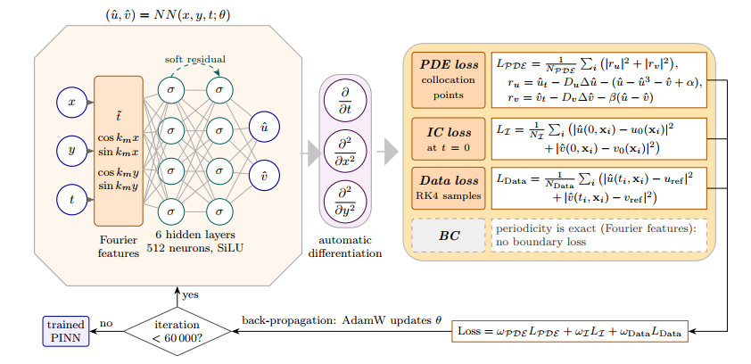
Architecture of the PINN with periodic feature embedding
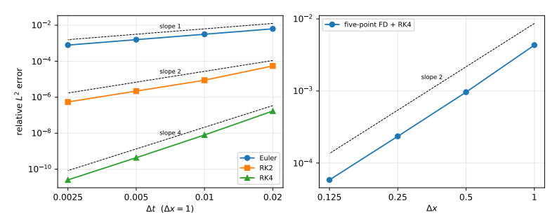
Temporal (left) and spatial (right) convergence of the finite-difference schemes; dashed lines indicate the theoretical slopes
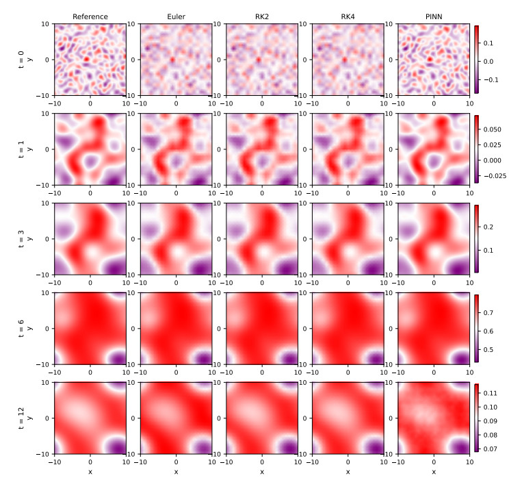
Spatiotemporal evolution of the excitation variable $ u $ obtained by different methods
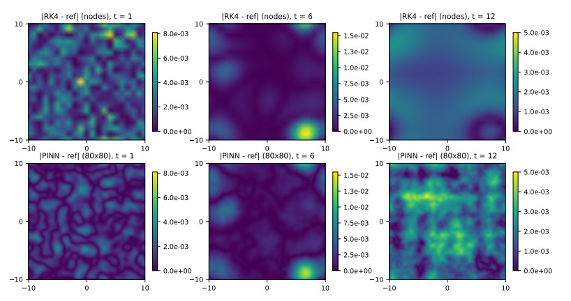
Absolute errors of $ u $ for RK4 (top) and the PINN (bottom)
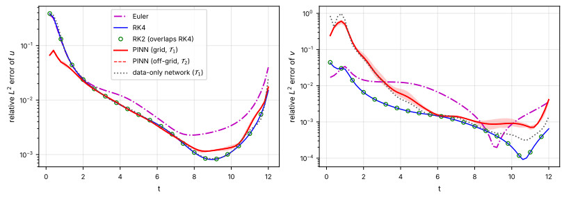
Relative $ L^2 $ errors of $ u $ (left) and $ v $ (right) versus time; the shaded band shows the range over three random seeds
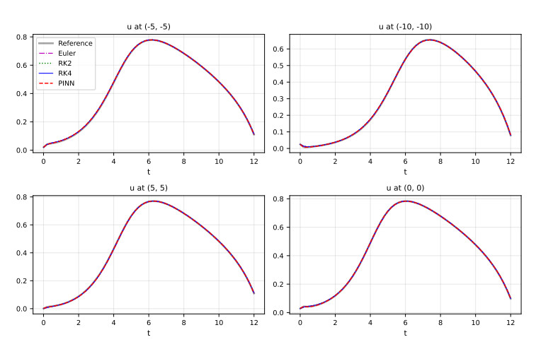
Temporal evolution of $ u $ at four spatial points
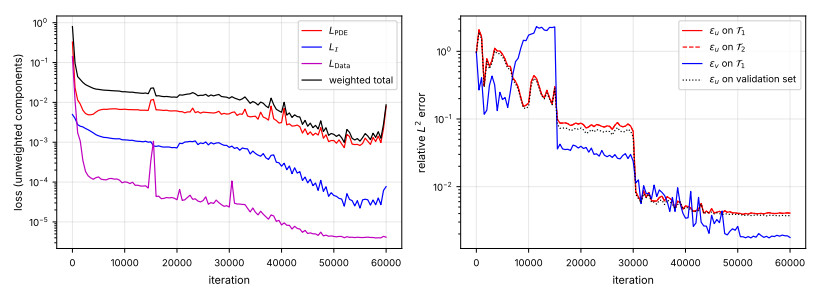
Training history of the PINN: loss components (left) and errors (right)
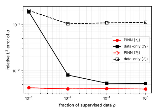
Relative $ L^2 $ error of $ u $ versus the fraction of supervised data





 DownLoad: