
Citation: Robert Ugochukwu Onyeneke, Chinyere Augusta Nwajiuba, Chukwuemeka Chinonso Emenekwe, Anurika Nwajiuba, Chinenye Judith Onyeneke, Precious Ohalete, Uwazie Iyke Uwazie. Climate change adaptation in Nigerian agricultural sector: A systematic review and resilience check of adaptation measures[J]. AIMS Agriculture and Food, 2019, 4(4): 967-1006. doi: 10.3934/agrfood.2019.4.967
[1] | Sijie Lu, Juan Xie, Yang Li, Bin Yu, Qin Ma, Bingqiang Liu . Identification of lncRNAs-gene interactions in transcription regulation based on co-expression analysis of RNA-seq data. Mathematical Biosciences and Engineering, 2019, 16(6): 7112-7125. doi: 10.3934/mbe.2019357 |
[2] | Yunxiang Wang, Hong Zhang, Zhenchao Xu, Shouhua Zhang, Rui Guo . TransUFold: Unlocking the structural complexity of short and long RNA with pseudoknots. Mathematical Biosciences and Engineering, 2023, 20(11): 19320-19340. doi: 10.3934/mbe.2023854 |
[3] | Mingshuai Chen, Xin Zhang, Ying Ju, Qing Liu, Yijie Ding . iPseU-TWSVM: Identification of RNA pseudouridine sites based on TWSVM. Mathematical Biosciences and Engineering, 2022, 19(12): 13829-13850. doi: 10.3934/mbe.2022644 |
[4] | Wangping Xiong, Yimin Zhu, Qingxia Zeng, Jianqiang Du, Kaiqi Wang, Jigen Luo, Ming Yang, Xian Zhou . Dose-effect relationship analysis of TCM based on deep Boltzmann machine and partial least squares. Mathematical Biosciences and Engineering, 2023, 20(8): 14395-14413. doi: 10.3934/mbe.2023644 |
[5] | Virgínia Villa-Cruz, Sumaya Jaimes-Reátegui, Juana E. Alba-Cuevas, Lily Xochilt Zelaya-Molina, Rider Jaimes-Reátegui, Alexander N. Pisarchik . Quantifying Geobacter sulfurreducens growth: A mathematical model based on acetate concentration as an oxidizing substrate. Mathematical Biosciences and Engineering, 2024, 21(5): 5972-5995. doi: 10.3934/mbe.2024263 |
[6] | Pingping Sun, Yongbing Chen, Bo Liu, Yanxin Gao, Ye Han, Fei He, Jinchao Ji . DeepMRMP: A new predictor for multiple types of RNA modification sites using deep learning. Mathematical Biosciences and Engineering, 2019, 16(6): 6231-6241. doi: 10.3934/mbe.2019310 |
[7] | Chongyi Tian, Longlong Lin, Yi Yan, Ruiqi Wang, Fan Wang, Qingqing Chi . Photovoltaic power prediction based on dilated causal convolutional network and stacked LSTM. Mathematical Biosciences and Engineering, 2024, 21(1): 1167-1185. doi: 10.3934/mbe.2024049 |
[8] | Yuan Yang, Yuwei Ye, Min Liu, Ya Zheng, Guozhi Wu, Zhaofeng Chen, Yuping Wang, Qinghong Guo, Rui Ji, Yongning Zhou . Family with sequence similarity 153 member B as a potential prognostic biomarker of gastric cancer. Mathematical Biosciences and Engineering, 2022, 19(12): 12581-12600. doi: 10.3934/mbe.2022587 |
[9] | Shaoyu Li, Su Xu, Xue Wang, Nilüfer Ertekin-Taner, Duan Chen . An augmented GSNMF model for complete deconvolution of bulk RNA-seq data. Mathematical Biosciences and Engineering, 2025, 22(4): 988-1018. doi: 10.3934/mbe.2025036 |
[10] | Kimberlyn Roosa, Ruiyan Luo, Gerardo Chowell . Comparative assessment of parameter estimation methods in the presence of overdispersion: a simulation study. Mathematical Biosciences and Engineering, 2019, 16(5): 4299-4313. doi: 10.3934/mbe.2019214 |
Molecular biology research on the molecular basis of biological activity requires data. Biologists acquire these data by using approaches and technologies such as microarray and RNA-sequencing (RNA-seq) techniques. Microarray technology is used to detect the sequences of nucleic acids and simultaneously thousands of gene transcripts from samples [1]. RNA-seq is a sequencing technique that can show the existence and amount of RNA in a biological sample by using next generation sequencing. Both techniques produce a high-dimensioanal gene expression data matrix with rows that indicate genes, columns that indicate experimental conditions, and cells that indicate the expression of that gene under those conditions. Gene expression data are very important for acquiring knowledge about cells, but there are frequently missing values. These missing values are often caused by experimental errors such as hybridization failures in microarray datasets and missing read counts in RNA-seq datasets. However, further analysis of these datasets requires a complete data matrix. Therefore, missing-value imputation approaches that use coherence the data are needed.
Two well-known missing-value imputation methods are LLS and BPCA. BPCA estimates missing values in the target gene (gene that contains missing values) by using a linear combination of principal components with parameters estimated using a Bayesian method. LLS uses a linear combination of the target gene and its similar genes to estimate the missing values in the target gene, and it uses clustering to measure gene similarities. In reality, genes are similar only under certain experimental conditions, so this similarity should only be measured by considering the related experimental conditions instead of all of the conditions. This is why clustering should be performed in rows and columns simultaneously, which is called biclustering [2]. Biclustering aims to identify local patterns in genes and conditions at the same time. The output of the biclutering technique is biclusters [3]. The use of this technique in LLS gives a better estimation of the missing values. Biclustering collates genes and conditions based on a weighted distance and correlation, respectively. Then, a regression model is used for least square-based missing-value estimation. An iterative framework is applied to improve the selection of coherent genes and correlated conditions. This method is called iterative bicluster-based least squares or bi-iLS [4].
Bi-iLS uses the row average to fill in all of the missing values in the target gene to obtain a temporary complete matrix. However, the row average is viewed as being flawed. The row average cannot reflect the real structure of the dataset because it only uses the information from an individual row. Thus, BPCA is considered better than the row average due to it reflecting the global covariance structure in all genes [5]. In this study, BPCA was used to obtain the temporary complete matrix in bi-iLS instead of the row average. This modification resulted in a new imputation method called bi-BPCA-iLS.
In this paper, the framework and implementation of our proposed bi-BPCA-iLS algorithm for missing-value imputation has been presented. The proposed missing-value imputation method will be implemented on a microarray dataset of Saccharomyces cerevisiae and an RNA-seq dataset of Schizosaccharomyces pombe.
In theory, every data point has a probability of being missing. The process of setting this probability is called the missing-data mechanism or response mechanism, while the models of these processes are called missing-data or response models [6,7,8,9]. Missing values can be categorized into three groups [10]. If the probability of a data point becoming missing is the same for all, then the missing values are called missing completely at random (MCAR). If the probability of a data point becoming missing is the same only for certain groups based on observational data, then the missing values are called missing at random (MAR). If missing values are neither MCAR nor MAR, then they are called missing not at random (MNAR) or not missing at random (NMAR). In other words, missing values in NMAR are independent of unobserved data [11].
Clustering is a technique that groups data points into several groups or clusters. In gene expression data, the purpose of clustering is to group genes into clusters where each cluster consists of genes that are similar to each other and dissimilar to genes from other clusters [12]. Biclustering in gene expression data is the simultaneous clustering of rows and columns [13]. The aim of biclustering is to find groups of similar genes based only on correlated experimental conditions. The output of biclustering is a bicluster. Genes are similar under certain experimental conditions, so biclustering is preferable to clustering. A comparison of biclustering and clustering in two-dimensional gene expression data matrices can be seen in Figure 1 [14]. Figure 1(a) indicates a clustering technique of genes based on all conditions, while Figure 1(b) shows a biclustering technique of genes based only on correlative experimental conditions.
LLS is a missing-value imputation method that identifies tne coherent information in gene expression data. There are two steps to the LLS method. The first step is to select k similar genes using Euclidean distance. The second step is to estimate the missing values [16,17]. This neighbor-based imputation method suits datasets that have a structure with dominant local similarities and high complexity [18].
Let a matrix E be the expression matrix consisting of m genes and n conditions. Assuming that the gene g1 has k similar genes (gs1, gs2, …, gsk) given the Euclidean distance and p missing values in the first p conditions, then the target gene y can be defined.
(gsgs1gs2...gsk)=(αwBA)=(α1α2...αpw1w2...wn−pB1,1B1,2...B1,pA1,1A1,2...A1,n−pB2,1B2,2...B2,pA2,1A2,2...A2,n−p........................Bk1Bk2...BkpAk1Ak2...Ak,n−p), |
where α is a vector of 1×p consisting of p missing values, w is a vector of 1×(n−p) consisting of the non-missing values in the target gene and the matrices B and A are the k similar genes' corresponding columns with α and w, respectively. Vector X can be defined as the solution to the least squares problem with AT and w.
||ATx−wT||. |
The solution of this least squares problem is
ˆx=(AAT)−1AwT=(AT)+wT, |
where A+ is the pseudoinverse of the matrix A. Hence, the missing values in the target gene g1 can be estimated using
ˆa=BTˆx=BT(AT)+w. |
To choose the proper value of k, LLS uses a heuristic algorithm by applying artificial missing values to genes. These artificial missing values will be estimated using different values of k, then the value of k that produces the lowest estimation error will be chosen as the proper value of k [16].
Bi-iLS is updated from the imputation method called LLS [16] in two aspects, i.e., the use of biclustering and an iterative framework. Bi-iLS can recognize gene similarities only under certain correlative conditions (biclustering), while LLS takes account all of the conditions in a data matrix. This makes bi-iLS preferable to LLS for gene expression data [4]. This imputation method suits data that have a dominant local similarity structure [18]. There are two parameters that need to be defined in the early stage of this process, namely k (for k similar genes) and T0.
Let the matrix E be the expression matrix consisting of m genes and n conditions. A gene that has p missing values is called the target gene. Assuming that all p missing values are in the first p conditions without a loss of generality, the target gene is defined as
gTt=(αw), |
where α is a vector of 1×p comprising p missing values and w is a vector of 1×(n−p) consisting of the non-missing values in the target gene. Similar to LLS, the first step of bi-iLS is to select k similar genes of target genes by using the Euclidean distance. The measurement of Euclidean distance requires a complete matrix, so bi-iLS uses the row average to fill n all of the missing values and obtain the temporary complete matrix. After selecting k similar genes, they are defined as
(gTs1...gTsk)=(BA), |
where g(s1)T denotes k similar genes, while the matrices B and A denote, respectively, the expression values for the first p conditions and remaining (n−p) conditions of the selected similar genes. Every condition has a different correlation with the other conditions. So, to account for the correlation or weight of each condition in the identification of the missing values, matrix R is defined as
R=BTA. |
Matrix R, with the size of p×(n−p), represents the weighted correlations between other conditions and the condition where the missing values in the target gene are found. The (j,v)th element of R is denoted by rj(v). The larger the value of rj(v), the larger are the weights and stronger are the correlations between the conditions with the missing values. Then, using R, k similar genes are reselected. Reselection of the k similar genes uses the weighted Euclidean distance of the target gene gt and other genes gs based on the location of the jth missing values. The equation is
dj(gt,gs)=√∑nv=p+1rj(v−p)2[gt(v)−gs(v)]2√∑nv=p+1rj(v)2, |
where g(v) denotes the vth element of gt or gs. Then, upon estimating the jth missing values for the target gene, conditions that are uncorrelated are removed from the least squares framework. Let
rj,max=maxv∈1,...,n−p|rj(v)|; |
then the conditions are said to be related if
|rj(v)|≥T0⋅rj,max. |
where T0 is a pre-defined parameter using the same heuristic algorithm to find the proper value of k. The removal of uncorrelated conditions redefines matrices A and B and w. Hence, we have
gTt=(αjwj), |
where αj denotes the jth missing values and wj denotes the non-missing values of correlated conditions. Also, we have
(gTs1...gTsk)=(BjAj), |
where Bj represents the jth columns of the data and Aj denotes a matrix consisting of the correlated columns of the k similar genes. Similar to LLS, a regression model αj=BTjxj is needed to estimate the jth missing value where xj contains the regression coefficient for k similar genes. xj can be obtained by minimizing the least squares error, as follows:
||ATx−wT||. |
Thus, the jth missing value in the target gene can be estimated by using
αj=BTjˆxj=BTj(AT)+jwTj, |
where (AT)+j is the pseudoinverse of ATj.
An iterative framework is applied to improve the selection of similar genes. A complete matrix output from the ith iteration will be the temporary complete matrix in the (i+1)th iteration. This iteration process will be repeated until it reaches the maximum iteration or a specific criterion. The complete framework of bi-iLS can be seen in Figure 2.
There are three main steps of the BPCA based imputation method: principal component (PC) regression, Bayesian estimation and application of an expectation-maximization (EM) repetitive algorithm [19]. In PC regression, Principal Component Analysis (PCA) represents the D-dimensional vector y as a linear combination of K principal axis vectors wl (1≤l≤K and K<D), as follows:
y=∑Kl=1xlwl+ϵ, |
where D is the quantity of columns in data, xl is a factor score and ∈ is the residual error. Assuming that there are no missing values, PCA can find wl=√λlul where λl and ul respectively denote the eigenvalues and eigenvectors of the corresponding covariance matrix of y. If missing values are present, then the principal axis vectors are split into two parts, i.e., W=(Wobs,Wmiss) where Wobs and Wmiss denote a matrix that has column vectors wobs1,…,wobsK and wmiss1,…,wmissK, respectively. Factor scores x=(x1,…,xK) are obtained by minimizing the residual error of the observed part as follows:
||yobs−Wobsx||2. |
This is a simple least squares problem that can be solved easily. Hence, the missing part of y can be estimated as
ymiss=Wmissx. |
However, these parameters are still unknown. BPCA uses a probabilistic PCA model under the assumption that the residual error ∈ and xl (1≤l≤K) obey normal distributions. The parameters W, μ and τ form a parameter set θ≡{W,μ,τ}. BPCA uses Bayesian estimation to estimate these parameters. It is used here because it can locate the best dimensions for latent space. This estimation is done by applying the EM algorithm until convergence is reached. This imputation method is appropriate for data with lower complexity structures [20].
The proposed bi-BPCA-iLS algorithm updates the bi-iLS algorithm during the process of obtaining the temporary complete matrix. Other than the process of obtaining the temporary complete matrix, bi-BPCA-iLS and bi-iLS are the same. In bi-ILS, the row average is used to fill in all of the missing values for the target genes to obtain a temporary complete matrix. However, the use of the row average to fill in the missing values is considered unsatisfactory. Row averages cannot reflect the structure of the data because they only use the information of a single row or gene [21]. Also, use of the row average is not an effective approach when there is an outlier in the target gene. Hence, the use of BPCA to get a temporary complete matrix is thought to be better than the use of the row average. BPCA can reflect the global covariance structure of all genes [5]. The main idea behind the proposed bi-BPCA-iLS method is to use BPCA instead of the row average to get a temporary complete matrix in the bi-iLS framework. This alteration means that bi-BPCA-iLS becomes an updated and improved missing-value imputation method. As mentioned before, bi-iLS matched to data that have a dominant local similarity structure and high complexity, while BPCA suits data with a structure of lower complexity. The idea of combining BPCA with bi-iLS makes bi-BPCA-iLS become more robust for data with a lower complexity structure. The complete framework of bi-BPCA-iLS can be seen in Figure 3. The differences table for the LLS, bi-iLS and bi-BPCA-iLS methods is given as Table 1.
LLS | Bi-iLS | Bi-BPCA-iLS | |
Gene similarity | Clustering | Biclustering | Biclustering |
Temporary complete matrix | Row-average | Row-average | BPCA |
Parameters | k | k and T0 | k and T0 |
Process of iteration | No | Yes | Yes |
Authors | Kim et al.[16] | Cheng et al.[4] | Newly Proposed |
Table 1 shows the differences between the three least squares-based imputation algorithms. LLS uses clustering to measure gene similarity, while bi-iLS and bi-BPCA-iLS use biclustering, which, as mentioned before, is considered to have higher efficacy. The row average is used in LLS and bi-iLS to obtain the temporary complete matrix, while bi-BPCA-iLS uses BPCA. Only bi-iLS and bi-BPCA-iLS iterates the imputation process. Our proposed imputation algorithm is the newest among these.
The proposed method has been implemented and evaluated on two-dimensional gene expressions: a microarray dataset and an RNA-seq dataset [22]. Bi-iLS was proven to perform well on the microarray datasets of Spellman 1998 for Saccharomyces cerevisiae [4], so bi-BPCA-iLS was also implemented on this dataset to make a performance comparison. Also, both bi-BPCA-iLS and bi-iLS were implemented on RNA-seq to analyze their performances on different gene expression datasets.
The microarray dataset is a cell cycle expression dataset for the yeast Saccharomyces cerevisiae; it has been synchronized using a CDC15 temperature-sensitive mutant [23]. According to Spellman et al., the samples of mRNA were taken every 10 minutes for 300 minutes. However, there were several missing time points in the published data. In fact, samples were taken every 20 minutes from 10 min to 70 min, and then every 10 minutes from 70 min to 250 min and every 20 minutes from 250 min to 290 min. Therefore, the CDC15 dataset contains the expression level of 6178 genes at 24 different time points which gives a matrix size of 6178 × 24. An example of the CDC15 dataset is shown in Table 2.
10 min | 30 min | 50 min | 70 min | … | 290 min | |
Gene 1 | −0.16 | 0.09 | −0.23 | 0.03 | … | −0.26 |
Gene 2 | NaN | NaN | NaN | −0.58 | … | NaN |
Gene 3 | −0.37 | −0.22 | -0.16 | 0.04 | … | −0.41 |
Gene 4 | NaN | NaN | NaN | −1.5 | … | NaN |
Gene 5 | −0.43 | −1.33 | −1.53 | −1.53 | … | 1.18 |
The CDC15 dataset had missing values, so genes that contained missing values were removed to get the ground truth. The ground truth was used to calculate the estimation error or NRMSE of each imputation methods. After removing genes that contained missing values, the size of the matrix became 4381 × 24. In the experiments for this dataset, r% of the observation values was set to be missing randomly where r = 1, 5, 10, 15, 20, 25 and 30. The estimation was repeated five times for each missing rate to generate the average result.
The RNA-seq dataset was gene expression data from the Schizosaccharomyces pombe or GSE150544 [24]. The technique of RNA sequencing was used to identify the differences between the gene expression levels of four different INO80 mutant strains, each with two replicates; this resulted in eight samples for each gene. The four strains were wt (control), Nht1, Iec1 and Iec5. The length for each gene, which indicates how many nucleotides are in that gene, was also included. In this experiment, only coding genes were observed. This dataset contained the expression of 5137 genes under nine different conditions, i.e., the length, wt_rep1, wt_rep2, nht1_rep1, nht1_rep2, Iec1_rep1, Iec2_rep2, Iec5_rep1 and Iec5_rep2, resulting in a matrix size of 5137 × 9. The data were not normalized to ensure the real expression of each gene and positive gene expression. An example of the GSE150544 dataset is shown in Table 3.
Length | wt_rep1 | wt_rep2 | nht1_rep1 | nht1_rep2 | Iec1_rep1 | Iec1_rep2 | Iec5_rep1 | Iec5_rep2 | |
Gene 1 | 669 | 18 | 16 | 8 | 2 | 4 | 15 | 17 | 19 |
Gene 2 | 993 | 46 | 50 | 45 | 25 | 33 | 34 | 25 | 29 |
Gene 3 | 3227 | 1623 | 1474 | 1655 | 1268 | 994 | 1870 | 1476 | 1849 |
Gene 4 | 868 | 258 | 322 | 215 | 200 | 138 | 284 | 278 | 286 |
Gene 5 | 2250 | 87 | 79 | 119 | 121 | 87 | 209 | 88 | 102 |
… | … | … | … | … | … | … | … | … | … |
Gene 5137 | 546 | 0 | 0 | 0 | 0 | 0 | 0 | 0 | 0 |
A value of zero indicates that a gene was not detected because the gene was not expressed, or was minimally expressed; therefore the value of zero is not a missing value. Then, r% of the observation values was set to be missing randomly where r = 1, 5, 10, 15, 20, 25 and 30. The estimation was repeated five times for each missing rate to generate the average result.
Our proposed imputation method was implemented in MATLAB. The parameters k and T0 were estimated automatically using the integrated function in our algorithm. The estimation process was iterated five times for each test. We carried out five tests for each missing rate to obtain the most accurate and convergent results. The imputation results applying our proposed method to the microarray dataset can be seen in Table 4 and Figure 4 below, where mr denotes the missing rate in Tables 4 and 5.
NRMSE Bi-BPCA-iLS | mr 1% | mr 5% | mr 10% | mr 15% | mr 20% | mr 25% | mr 30% |
Test 1 | 0.1851 | 0.3934 | 0.4766 | 0.5485 | 0.5681 | 0.6102 | 0.6369 |
Test 2 | 0.1685 | 0.4610 | 0.5101 | 0.5634 | 0.5717 | 0.6093 | 0.6269 |
Test 3 | 0.2065 | 0.3882 | 0.4888 | 0.5359 | 0.5887 | 0.6044 | 0.6206 |
Test 4 | 0.2170 | 0.3741 | 0.4892 | 0.5476 | 0.5839 | 0.6034 | 0.6300 |
Test 5 | 0.2371 | 0.3934 | 0.4811 | 0.5458 | 0.5801 | 0.6000 | 0.6203 |
Average | 0.20284 | 0.40202 | 0.48916 | 0.54824 | 0.5785 | 0.60546 | 0.62694 |
NRMSE Bi-BPCA-iLS | mr 1% | mr 5% | mr 10% | mr 15% | mr 20% | mr 25% | mr 30% |
Test 1 | 0.3020 | 0.2593 | 0.2226 | 0.2351 | 0.2470 | 0.2595 | 0.2612 |
Test 2 | 0.1317 | 0.1737 | 0.2684 | 0.2527 | 0.2518 | 0.2515 | 0.2493 |
Test 3 | 0.3011 | 0.2814 | 0.2577 | 0.2378 | 0.2364 | 0.2234 | 0.2641 |
Test 4 | 0.3976 | 0.2838 | 0.2273 | 0.2791 | 0.2872 | 0.2357 | 0.2457 |
Test 5 | 0.4162 | 0.1917 | 0.2571 | 0.2595 | 0.2589 | 0.2485 | 0.3046 |
Average | 0.30972 | 0.23798 | 0.24662 | 0.25284 | 0.25626 | 0.24372 | 0.26498 |
The imputation results of applying our proposed method to the RNA-seq dataset can be seen in Table 5 and Figure 5 below.
Based on Table 5 and Figure 5, the average value of the NRMSE for a missing rate of 1% was 0.29626, for a missing rate of 5% was 0.23798 and for a missing rate of 10% was 0.24662. The lowest estimation error was achieved when the missing rate was 5%; it was highest when the missing rate was 1%. The NRMSE values were predominantly below 0.3 at every missing rate, indicating that our proposed imputation method, bi-BPCA-iLS, performed well on the GSE150544 dataset.
Two existing methods, LLS and bi-iLS, were compared to our proposed imputation method. This comparison entailed the use of the the average value of NRMSE and computational time generated from five trials for every missing rate. The difference between the NRMSE values of Method A and Method B divided by the NRMSE value of Method A shows the improvement of Method B relative to Method A. If the improvement value is positive, then Method B results in a higher imputation accuracy compared to Method A. If the improvement value is negative, then method B has a decrease in imputation accuracy compared to Method A.
The averages of the improvement values across all missing rates for the CDC15 dataset are shown in Table 6 below. Based on these figures, the bi-iLS algorithm showed a significant overall improvement in NRMSE value (10.07%) relative to the LLS algorithm. Our proposed method, bi-BPCA-iLS, also showed a significant overall improvement in NRMSE value: 10.612% relative to LLS and 0.582% relative to bi-iLS.
Average value of NRMSE | NRMSE from LLS | NRMSE from Bi-iLS | NRMSE from Bi-BPCA-iLS | Improvement of bi-iLS relative to LLS | Improvement of bi-BPCA-iLS relative to LLS | Improvement of bi-BPCA-iLS relative to bi-iLS |
Missing rate 1% | 0.20938 | 0.20792 | 0.20284 | 0.697296781% | 3.123507498% | 2.443247403% |
Missing rate 5% | 0.51722 | 0.40444 | 0.40202 | 21.80503461% | 22.27292061% | 0.598358224% |
Missing rate 10% | 0.57694 | 0.49252 | 0.48916 | 14.63237078% | 15.2147537% | 0.682205799% |
Missing rate 15% | 0.61448 | 0.5499 | 0.54824 | 10.50969926% | 10.77984637% | 0.301873068% |
Missing rate 20% | 0.63408 | 0.5799 | 0.5785 | 8.544663134% | 8.765455463% | 0.241420935% |
Missing rate 25% | 0.65518 | 0.60512 | 0.60546 | 7.640648371% | 7.588754235% | -0.05618720% |
Missing rate 30% | 0.6708 | 0.62610 | 0.62694 | 6.663685152% | 6.538461538% | -0.13416387% |
Average improvement | 10.070% | 10.612% | 0.582% |
As shown in Table 6 and Figure 6, the imputation method that produced the lowest overall NRMSE across all missing rates for the CDC15 dataset was our proposed method, bi-BPCA-iLS.
After comparing the values of NRMSE, the computational times of the imputation methods were also compared in MATLAB. Based on Table 7, bi-iLS is shown to add an overall average of 320.134 seconds of computational time compared to LLS. bi-BPCA-iLS is shown to add an overall average of 343.850 seconds of computational time relative to LLS and only 23.716 seconds relative to bi-iLS.
Average computational time | Computational time of LLS | Computational time of Bi-iLS | Computational time of Bi-BPCA-iLS | Additional time of bi-iLS relative to LLS | Additional time of bi-BPCA-iLS relative to LLS | Additional time of bi-BPCA-iLS relative to bi-iLS |
Missingrate 1% | 60.402 | 120.439 | 126.396 | 60.037 | 65.994 | 5.957 |
Missingrate 5% | 76.419 | 255.455 | 275.087 | 179.036 | 198.668 | 19.632 |
Missingrate 10% | 71.727 | 388.521 | 455.319 | 316.794 | 383.592 | 66.798 |
Missingrate 15% | 59.123 | 378.844 | 444.281 | 319.721 | 385.158 | 65.437 |
Missingrate 20% | 52.033 | 472.843 | 434.815 | 420.81 | 382.782 | -38.028 |
Missingrate 25% | 45.539 | 457.156 | 467.654 | 411.617 | 422.115 | 10.498 |
Missingrate 30% | 61.047 | 593.972 | 629.689 | 532.925 | 568.642 | 35.717 |
Average additional computational time in seconds | 320.134 | 343.850 | 23.716 |
As shown in Figure 7, LLS displayed a consistent computational time for every missing rate, while bi-iLS and bi-BPCA-iLS had additional computational time following the increase in missing rates. In conclusion, the fastest imputation method was LLS; this is related to the high NRMSE it generated compared to the other methods. Regarding bi-iLS and bi-BPCA-iLS, there was no significant computational time difference between these two methods. If the goal is achieving a lower NRMSE, then one can use bi-BPCA-iLS instead of bi-iLS.
The average improvement values across all missing rates for the RNA-seq dataset (GSE150544) are shown in Table 8. We can see that the bi-iLS algorithm showed an overall improvement in NRMSE value of 5.12% relative to the LLS algorithm. Our proposed method, bi-BPCA-iLS, had an overall improvement in NRMSE value of 8.20% relative to LLS and 3.09% relative to bi-iLS.
Average value of NRMSE | NRMSE from LLS | NRMSE from Bi-iLS | NRMSE from Bi-BPCA-iLS | Improvement of bi-iLS relative to LLS | Improvement of bi-BPCA-iLS relative to LLS | Improvement of bi-BPCA-iLS relative to bi-iLS |
Missing rate 1% | 0.29318 | 0.32288 | 0.30972 | -10.1303% | -5.64159% | 4.075818% |
Missing rate 5% | 0.23604 | 0.25204 | 0.23798 | -6.77851% | -0.82189% | 5.57848% |
Missing rate 10% | 0.26032 | 0.25436 | 0.24662 | 2.28949% | 5.262754% | 3.042931% |
Missing rate 15% | 0.27980 | 0.26908 | 0.25284 | 3.831308% | 9.635454% | 6.03538% |
Missing rate 20% | 0.28308 | 0.25652 | 0.25626 | 9.382507% | 9.474354% | 0.101357% |
Missing rate 25% | 0.29156 | 0.24558 | 0.24372 | 15.77034% | 16.40829% | 0.757391% |
Missing rate 30% | 0.34442 | 0.27056 | 0.26498 | 21.44475% | 23.06486% | 2.062389% |
Average improvement | 5.12% | 8.20% | 3.09% |
The performances of LLS, bi-iLS, and bi-BPCA-iLS on the GSE1505544 data can be seen in Table 8. Bi-BPCA-iLS and bi-iLS had negative performances when the missing rate was 1% and 5%, so LLS performed well when the missing rate was below 5% in this dataset. But when the missing rate moved above 5%, the performance of bi-BPCA-iLS was superior to the other methods. As shown in Figure 8, the average NRMSE from bi-BPCA-iLS tended to be lower than those of the other methods.
After comparing the values of NRMSE, the computational times of the imputation methods were compared in MATLAB. Based on Table 9 and Figure 9, bi-iLS is shown to add an overall 117.200 seconds of computational time relative to LLS. While bi-BPCA-iLS is shown to add an overall 126.549 seconds of computational time relative to LLS and only 9.349 seconds relative to bi-iLS. There is no significant computational time difference between bi-BPCA-iLS and bi-iLS, only 9.349 seconds.
Average computational time | Computational time of LLS | Computational time of Bi-iLS | Computational time of Bi-BPCA-iLS | Additional time of bi-iLS relative to LLS | Additional time of bi-BPCA-iLS relative to LLS | Additional time of bi-BPCA-iLS relative to bi-iLS |
Missingrate 1% | 28.418 | 79.678 | 82.420 | 51.26 | 54.002 | 2.742 |
Missingrate 5% | 22.080 | 107.653 | 109.090 | 85.573 | 87.01 | 1.437 |
Missingrate 10% | 18.678 | 130.136 | 142.0635 | 111.458 | 123.3855 | 11.9275 |
Missingrate 15% | 25.831 | 155.458 | 158.179 | 129.627 | 132.348 | 2.721 |
Missingrate 20% | 22.429 | 160.494 | 165.366 | 138.065 | 142.937 | 4.872 |
Missingrate 25% | 20.513 | 152.178 | 189.796 | 131.665 | 169.283 | 37.618 |
Missingrate 30% | 25.018 | 197.769 | 201.895 | 172.751 | 176.877 | 4.126 |
Average additional computational time in seconds | 117.200 | 126.549 | 9.349 |
Early approaches toward missing-value imputation tended to consider all experimental conditions in measuring gene similarity. However, genes are only similar under certain experimental conditions. This meant that an bi-iLS algorithm for imputing missing values has to be developed. This algorithm uses the row average to obtain a temporary complete matrix, which has become to be considered as a flawed approach. The row average cannot reflect the real structure of the dataset because it only leverages the information of an individual row. Thus, in this study, we used BPCA to obtain a temporary complete matrix instead of using row average. The proposed algorithm is called bi-BPCA-iLS. After finding the temporary complete matrix using BPCA, the required parameters can be found. Our proposed algorithm performs clustering on genes and conditions alternately to find biclusters that consist of a subset of genes that are similar under a subset of conditions. After the biclusters related to the target genes are found, least squares estimation of the missing values can be performed while considering only related genes and conditions. This estimation process can be iterated to improve the selection of similar genes and conditions in every iteration, which improves the accuracy of the missing-value imputation.
Experiments were conducted on two gene expression datasets: a microarray dataset for Saccharomyces cerevisiae (CDC15) and an RNA-seq dataset for Schizosaccharomyces pombe (GSE150544). The results show that our proposed method is best suited to impute missing values in microarray datasets and RNA-seq datasets based on the NRMSE, compared to preceding imputation methods such as LLS and bi-iLS. Significant NRMSE improvements of 10.612% for CDC15 and 8.20% for GSE150544 were observed when using bi-BPCA-iLS instead of LLS, indicating the importance of using biclustering and iterative frameworks. Also, bi-BPCA-iLS showed NRMSE improvements of 0.582% for CDC15 and 3.09% for GSE150544 relative to bi-iLS, indicating that the temporary complete matrix is better obtained with BPCA rather than via the row average. The additional computational time of bi-BPCA-iLS compared to bi-iLS was only 23.716 seconds for CDC15 and 9.349 seconds for GSE150544, which can be concluded as not significant. These experimental results show that our proposed method outperforms the other two existing methods. Thus, our proposed method is applicable to other datasets that fit our assumption.
The missing-value imputation method bi-BPCA-iLS outperformed other methods such as LLS and bi-iLS in selected microarray and RNA-seq datasets in terms of the NRMSE. The improvement relative to LLS indicates the importance of using biclustering and iterative framework in the imputation, while the improvement relative to bi-iLS indicates that the temporary complete matrix is better obtained with BPCA rather than via the row average.
Universitas Indonesia funded this research with grant number NKB-030/UN2.F3/HKP.05.00/2021.
The authors declare that there is no conflict of interest.
[1] | IPCC (2014) Climate Change 2014: Impacts, adaptation, and vulnerability-Contribution of Working Group II to the Fifth Assessment Report of the Intergovernmental Panel on Climate Change. Cambridge, United Kingdom: Cambridge University Press. |
[2] | IPCC (2014) Climate Change 2014: Synthesis Report. Geneva, Switzerland: Intergovernmental Panel on Climate Change. Retrieved July 1, 2019, Available from: https://www.ipcc.ch/site/assets/uploads/2018/05/SYR_AR5_FINAL_full_wcover.pdf. |
[3] |
Abidoye BO, Kurukulasuriya P, Mendelsohn R (2017) South-East Asian farmer perceptions of climate change. Clim Change Econ 8: 1740006. doi: 10.1142/S2010007817400061
![]() |
[4] |
Konchar KM, Staver B, Salick J, et al. (2015) Adapting in the shadow of Annapurna: a climate tipping point. J Ethnobiol 35: 449-471. doi: 10.2993/0278-0771-35.3.449
![]() |
[5] | Aldunce P, Handmer J, Beilin R, et al. (2016) Is climate change framed as 'business as usual' or as a challenging issue? The practitioners' dilemma. Environ Plann 34: 999-1019. |
[6] | Scheffers BR, Meester L, Bridge TC, et al. (2016) The broad footprint of climate change from genes to biomes to people. Science 354: 6313. |
[7] |
Voccia A (2012) Climate change: What future for small, vulnerable states? Int J Sust Dev World Ecol 19: 101-115. doi: 10.1080/13504509.2011.634032
![]() |
[8] |
Spires M, Shackleton S, Cundill G (2014) Barriers to implementing planned community-based adaptation in developing countries: A systematic literature review. Clim Dev 6: 277-287. doi: 10.1080/17565529.2014.886995
![]() |
[9] | Bockel L, Vian L, Torre C (2016) Towards sustainable impact monitoring of green agriculture and forestry investments by NDBs: Adapting MRV methodology. Rome, Italy: Food and Agriculture Organization. |
[10] |
Glenn A, James WE, Fuller RA (2016) Global mismatch between greenhouse gas emissions and the burden of climate change. Sci Rep 6: 20281. doi: 10.1038/srep20281
![]() |
[11] |
Jackson G, McNamara K, Witt B (2017) A framework for disaster vulnerability in a small island in the Southwest Pacific: A case study of Emae Island, Vanuatu. Int J Disaster Risk Sci 8: 358-373. doi: 10.1007/s13753-017-0145-6
![]() |
[12] |
Easterling WE (1996) Adapting North American agriculture to climate change in review. Agric For Meteorol 80: 1-53. doi: 10.1016/0168-1923(95)02315-1
![]() |
[13] | FAO (2007) Adaptation to climate change in agriculture, forestry and fisheries: Perspective, framework and priorities. Rome: Food and Agriculture Organization. |
[14] |
Berrang-Ford L, Pearce T, Ford JD (2015) Systematic review approaches for climate change adaptation research. Reg Environ Chang 15: 755-769. doi: 10.1007/s10113-014-0708-7
![]() |
[15] | Ifejika-Speranza C (2010) Resilient adaptation to climate change in African Agriculture. Bonn: Deutsches Institut für Entwicklungspolitik (DIE). |
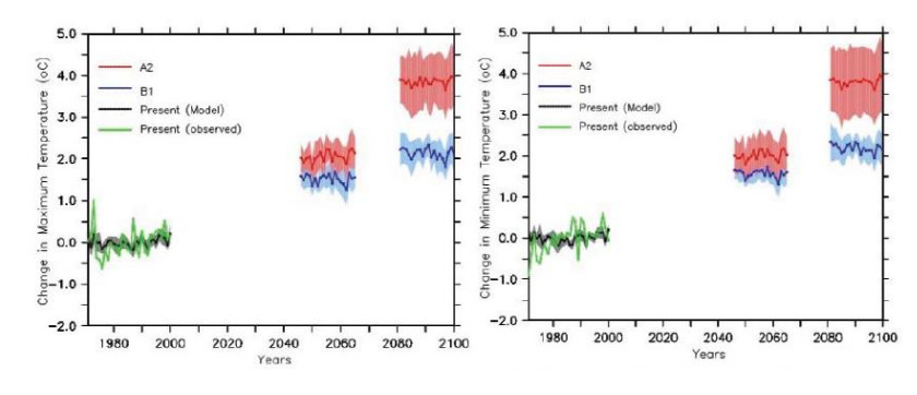
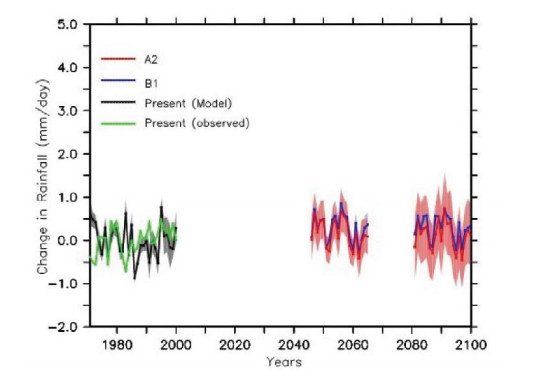
[16] | Abiodun BJ, Salami AT, Tadross M (2011) Climate change scenarios for Nigeria: Understanding biophysical impacts. Ibadan, Nigeria: Building Nigeria's Response to Climate Change (BNRCC) Project. |
[17] | IPCC (2018) Global warming of 1.5 ℃ Geneva, Switzerland: Intergovernmental Panel on climate change. |
[18] | NBS (2017) Nigerian Gross Domestic Product Report, Abuja, Nigeria: National Bureau of Statistics. |
[19] | Yakubu MM, Akanegbu BN (2015) The Impact of international trade on economic growth in Nigeria: 1981-2012. Eur J Bus Econ Account 3: 26-36. |
[20] |
Berg A, de Noblet-Ducoudre N, Benjamin S, et al. (2013) Projections of climate change impacts on potential C4 crop productivity over tropical regions. Agric For Meteorol 170: 89-102. doi: 10.1016/j.agrformet.2011.12.003
![]() |
[21] | Mereu V, Santini M, Cervigni R, et al (2018) Robust decision making for a climate-resilient development of the agricultural sector in Nigeria. In: Lipper L, McCarthy N, Zilberman D, et al., Eds., Climate Smart Agriculture: Building Resilience to Climate Change, Rome, Italy: Food and Agriculture Organization of the United Nations (FAO), 277-306. |
[22] | Adejuwon JO (2005) Food crop production in Nigeria. Present effects of climate variability. Clim Res 30: 53-60. |
[23] |
Odekunle TO (2004) Rainfall and the length of the growing season in Nigeria. Int J Climatol 24: 467-479. doi: 10.1002/joc.1012
![]() |
[24] |
Remling E, Veitayaki J (2016) Community-based action in Fiji's Gau Island: A model for the Pacific? Int J Clim Chang Str Manage 8: 375-398. doi: 10.1108/IJCCSM-07-2015-0101
![]() |
[25] | Ogbo A, Lauretta NE, Ukpere W (2013) Risk management and challenges of climate change in Nigeria. J Hum Ecol 41: 221-235. |
[26] |
Obioha EE (2008) Climate change, population drift and violent conflict over land resources in Northeastern Nigeria. J Hum Ecol 23: 311-324. doi: 10.1080/09709274.2008.11906084
![]() |
[27] |
Mburu BM, Kung'u JB, Muriuku JN (2015) Climate change adaptation strategies by small-scale farmers in Yatta District, Kenya. Afr J Environ Sci Technol 9: 712-722. doi: 10.5897/AJEST2015.1926
![]() |
[28] | Cooper C, Booth A, Varley-Campbell J, et al. (2018) Defining the process to literature searching in systematic reviews: A literature review of guidance and supporting studies. BMC Med Res Methodol 85: 1-14. |
[29] |
Babatunde KA, Begum RA, Said FF (2017) Application of computable general equilibrium (CGE) to climate change mitigation policy: A systematic review. Renew Sust Energ Rev 78: 61-71. doi: 10.1016/j.rser.2017.04.064
![]() |
[30] |
Escarcha JF, Lassa JA, Zander KK (2018) Livestock under climate change: A systematic review of impacts and adaptation. Climate 6: 54. doi: 10.3390/cli6030054
![]() |
[31] |
Folke C (2006) Resilience: The emergence of a perspective for social-ecological systems analyses. Global Environ Chang 16: 253-267. doi: 10.1016/j.gloenvcha.2006.04.002
![]() |
[32] |
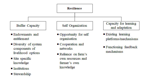
Ifejika-Speranza C (2013) Buffer capacity: Capturing a dimension of resilience to climate change in African smallholder agriculture. Reg Environ Chang 13: 521-535. doi: 10.1007/s10113-012-0391-5
![]() |
[33] |
Pretty J (2008) Agricultural sustainability: Concepts, principles and evidence. Philos Trans R Soc Lond B Biol Sci 363: 447-465. doi: 10.1098/rstb.2007.2163
![]() |
[34] | Dorward A, Anderson S, Clark S (2001) Asset functions and livelihood strategies: A framework for pro-poor analysis, policy and practice. Imperial College at Wye, Department of Agricultural Sciences: ADU Working Papers 10918. |
[35] |
Shaffril HA, Krauss SE, Samsuddin SF (2018) A systematic review on Asian's farmers' adaptation practices towards climate change. Sci Total Environ 644: 683-695. doi: 10.1016/j.scitotenv.2018.06.349
![]() |
[36] |
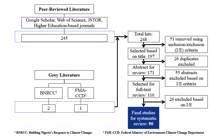
Moher D, Liberati A, Tetzlaff J, et al. (2009) Preferred reporting items for systematic reviews and meta-analyses: The PRISMA statement. PLoS Med 6: e1000097. doi: 10.1371/journal.pmed.1000097
![]() |
[37] | Singh C, Deshpande T, Basu R (2017) How do we assess vulnerability to climate change in India? A systematic review of literature. Reg Environ Chang 17: 527-538. |
[38] |
Rusinamhodzi L, Corbeels M, Nyamangara J, et al. (2012) Maize-grain legume intercropping is an attractive option for ecological intensification that reduces climatic risk for smallholder farmers in central Mozambique. Field Crops Res 136: 12-22. doi: 10.1016/j.fcr.2012.07.014
![]() |
[39] |
Challinor A, Wheeler T, Garfoth C, et al. (2007) The vulnerability of food crop systems in Africa to climate change. Clim Chang 83: 381-399. doi: 10.1007/s10584-007-9249-0
![]() |
[40] |
Morton JF (2007) The impact of climate change on smallholder and subsistence agriculture. Proc Natl Acad Sci USA 104: 19680-19685. doi: 10.1073/pnas.0701855104
![]() |
[41] |
Armbrecht I, Gallego-Ropero MC (2007) Testing ant predation on the coffee berry borer in shaded and sun coffee plantations in Colombia. Entomol Exp Appl 124: 261-267. doi: 10.1111/j.1570-7458.2007.00574.x
![]() |
[42] |
Lin BB (2011) Resilience in agriculture through crop diversification: Adaptive management for environmental change. BioScience 61: 183-193. doi: 10.1525/bio.2011.61.3.4
![]() |
[43] | Grubben G, Klaver W, Nono-Womdim R, et al. (2014) Vegetables to combat the hidden hunger in Africa. Chronica Hort 54: 24-32. |
[44] | Luoh JW, Begg CB, Symonds RC, et al. (2014) Nutritional yield of African indigenous vegetables in water-deficient and water-sufficient conditions. Food Nutri Sci 5: 812-822. |
[45] |
Lunduka RW, Mateva KL, Magoroshoko C, et al. (2019) Impact of adoption of drought-tolerant maize varieties on total maize production in south Eastern Zimbabwe. Clim Dev 11: 35-46. doi: 10.1080/17565529.2017.1372269
![]() |
[46] | Akinnagbe OM, Irohibe IJ (2014) Agricultural adaptation strategies to climate change impacts in Africa: A review. Bangladesh J Agric Res 39: 407-418. |
[47] |
Waha K, Müller C, Bondeau A, et al. (2013) Adaptation to climate change through the choice of cropping system and sowing date in sub-Saharan Africa. Global Environ Chang 23: 130-143. doi: 10.1016/j.gloenvcha.2012.11.001
![]() |
[48] | Atedhor GO (2015) Strategies for agricultural adaptation to climate change in Kogi state, Nigeria. Ghana J Geogr 7: 20-37. |
[49] |
Westengen OT, Brysting AK (2014) Crop adaptation to climate change in the semi-arid zone in Tanzania: The role of genetic resources and seed systems. Agri Food Secur 3: 1-12. doi: 10.1186/2048-7010-3-1
![]() |
[50] | Sanz MJ, de Vente J, Chotte JL, et al. (2017) Sustainable land management contribution to successful land-based climate change adaptation and mitigation: A report of the science-policy interface. Bonn, Germany: United Nations Convention to Combat Desertification (UNCCD). |
[51] | FAO (2017) Voluntary guidelines for sustainable soil management. Rome, Italy: Food and Agriculture Organization. |
[52] |
Stavi I (2013) Biochar use in forestry and tree-based agro-ecosystems for increasing climate change mitigation and adaptation. Int J Sust DevWorld Ecol 20: 166-181. doi: 10.1080/13504509.2013.773466
![]() |
[53] |
Lal R (2015) Sequestering carbon and increasing productivity by conservation agriculture. J Soil Water Conserv 70: 55-62. doi: 10.2489/jswc.70.3.55A
![]() |
[54] |
Stavi I, Bel G, Zaady E (2016) Soil functions and ecosystem services in conventional, conservation, and integrated agricultural systems. A review. Agron Sustain Dev 36: 1-12. doi: 10.1007/s13593-015-0343-9
![]() |
[55] |
Agbonlahor MU, Aromolaran AB, Aiboni VI (2003) Sustainable soil management practices in small farms of southern Nigeria: A poultry-food crop integrated farming approach. J Sustain Agric 22: 51-62. doi: 10.1300/J064v22n04_05
![]() |
[56] | Thierfelder C, Matemba-Mutasa R, Rusinamhodzi L (2015) Yield response of maize (Zea mays L.) to conservation agriculture cropping system in Southern Africa. Soil Till Res 146: 230-242. |
[57] | Oyekale AS, Oladele OI (2012) Determinants of climate change adaptation among cocoa farmers in Southwest Nigeria. ARPN J Sci Technol 2: 154-168. |
[58] |
Merrey DJ, Sally H (2008) Micro-AWM Technologies for food security in Southern Africa: Part of the solution or a red herring? Water Policy 10: 515-530. doi: 10.2166/wp.2008.025
![]() |
[59] | CGIAR (2016) Agricultural practices and technologies to enhance food security, resilience and productivity in a sustainable manner: Messages to SBSTA 44 agriculture workshops, CCAFS Working Paper no. 146, Copenhagen, Denmark, 2016. |
[60] |
Abraham TW, Fonta WM (2018) Climate change and financing adaptation by farmers in northern Nigeria. Financ Innov 4: 11. Available from: https://doi.org/10.1186/s40854-018-0094-0. doi: 10.1186/s40854-018-0094-0
![]() |
[61] | BNRCC (2011) Reports of pilot projects in community-based adaptation to climate change in Nigeria. Ibadan, Nigeria: Building Nigeria's Response to Climate Change (BNRCC) Project. |
[62] |
Asfaw A, Simane B, Hassen A, et al. (2017) Determinants of non-farm livelihood diversification: Evidence from rainfed-dependent smallholder farmers in Northcentral Ethiopia (Woleka sub-basin). Dev Stud Res 4: 22-36. doi: 10.1080/21665095.2017.1413411
![]() |
[63] | Nzegbule EC, Nwajiuba C, Ujor G, et al. (2019) Sustainability and the effectiveness of BNRCC community-based adaptation (CBA) to address climate change impact in Nigeria. In: Leal FW Eds., Handbook of Climate Change Resilience, Cham: Springer, 1-22. |
[64] |
Akrofi-Atitianti F, Ifejika-Speranza C, Bockel L, et al. (2018) Assessing climate smart agriculture and its determinants of practice in Ghana: A case of the cocoa production system. Land 7: 30. doi: 10.3390/land7010030
![]() |
[65] | Adepoju AO, Osunbor PP (2018) Small scale poultry farmers' choice of adaption strategies to climate change in Ogun State, Nigeria. Rural Sustain Res 40: 32-40. |
[66] | Salem BH, López-Francos A (2012) Feeding and management strategies to improve livestock productivity, welfare and product quality under climate change. 14th International Seminar of the Sub-Network on Nutrition of the FAO-CIHEAM Inter-Regional Cooperative Research and Development Network on Sheep and Goats. Hammamet, Tunisia. |
[67] | IAEA (2010) Improving livestock production using indigenous resources and conserving the environment. Vienna, Austria: International Atomic Energy Agency. |
[68] | Lamy E, van Harten S, Sales-Baptista E, et al. (2012) Factors influencing livestock productivity. In: Sejian V, Naqvi SM, Ezeji T, et al. Eds., Environmental Stress and Amelioration in Livestock Production, Berlin, Germany: Springer, 19-51. |
[69] | Gebremedhin B, Hoekstra D, Jemaneh S (2007) Heading towards commercialization? The case of live animal marketing in Ethiopia. Nairobi, Kenya: Improving Productivity and Market Success (IPMS) of Ethiopian Farmers. Working Paper 5. ILRI (International Livestock Research Institute). |
[70] | Batima P (2006) Climate change vulnerability and adaptation in the livestock sector of Mongolia. Washington, DC: Assessments of Impacts and Adaptations to Climate Change (AIACC), Project No. AS 06. |
[71] | Okonkwo WI, Akubuo CO (2001) Thermal analysis and evaluation of heat requirement of a passive solar energy poultry chick brooder. Nig J Renew Energ 9: 83-87. |
[72] |
Nyoni NM, Grab S, Archer ER (2019) Heat stress and chickens: Climate risk effects on rural poultry farming in low-income countries. Clim Dev 11: 83-90. doi: 10.1080/17565529.2018.1442792
![]() |
[73] |
Elijah OA, Adedapo A (2006) The effect of climate on poultry productivity in Ilorin Kwara State, Nigeria. Int J Poult Sci 5: 1061-1068. doi: 10.3923/ijps.2006.1061.1068
![]() |
[74] | Ampaire A, Rothschild MF (2010) Effects of training and facilitation of farmers in Uganda on livestock development. Livest Res Rural Dev 22: 1-7. |
[75] | Shelton C (2014) Climate change adaptation in fisheries and aquaculture: Compilation of initial examples. FAO Fisheries and Agriculture Circular No. 1088. Rome: Food and Agriculture Organization. |
[76] |
Ficke AD, Myrick CA, Hansen LJ (2007) Potential impacts of global climate change on freshwater fisheries. Rev Fish Biol Fisher 17: 581-613. doi: 10.1007/s11160-007-9059-5
![]() |
[77] | Nwabeze GO, Erie AP, Erie GO (2012) Fishers' adaptation to climate change in the Jebba Lake Basin, Nigeria. J Agric Ext 16: 68-78. |
[78] | Adebayo OO (2012) Climate change perception and adaptation strategies on catfish farming in Oyo State, Nigeria. Glob J Sci Frontier Res Agric Vet Sci 12: 1-7. |
[79] | Huq S, Reid H (2007) Community-based adaptation: A vital approach to the threat climate change poses to the poor. London: International Institute for Environment and Development. |
[80] | Achoja FO, Oguh VO (2018) Income effect of climate change adaptation technologies among crop farmers in Delta State, Nigeria. Int J Agric Rural Dev 21: 3611-3616. |
[81] | Agomuo CI, Asiabaka CC, Nnadi FN, et al. (2015) Rural women farmers' use of adaptation strategies to climate change in Imo State. Nigeria Int J Agric Rural Dev 18: 2305-2310. |
[82] | Ajayi JO (2015) Adaptation strategies to climate change by farmers in Ekiti State, Nigeria. Appl Trop Agric 20: 01-07. |
[83] | Ajieh PC, Okoh RN (2012) Constraints to the implementation of climate change adaptation measures by farmers in delta state, Nigeria. Glob J Sci Frontier Res Agric Vet Sci 12: 1-7. |
[84] | Akinbile LA, Oluwafunmilayo AO, Kolade RI (2018) Perceived effect of climate change on forest dependent livelihoods in Oyo State, Nigeria. J Agric Ext 22: 169-179. |
[85] | Akinwalere BO (2017) Determinants of adoption of agroforestry practices among farmers in Southwest Nigeria. Appl Trop Agric 22: 67-72. |
[86] | Anyoha NO, Nnadi FN, Chikaire J, et al. (2013) Socio-economic factors influencing climate change adaptation among crop farmers in Umuahia South Area of Abia State, Nigeria. Net J Agric Sci 1: 42-47. |
[87] | Apata TG (2011) Factors influencing the perception and choice of adaptation measures to climate change among farmers in Nigeria: Evidence from farm households in Southwest Nigeria. Environ Econ 2: 74-83. |
[88] | Arimi K (2014) Determinants of climate change adaptation strategies used by rice farmers in Southwestern, Nigeria. J Agr Rural Dev Trop 115: 91-99. |
[89] | Asadu AN, Ozioko RI, Dimelu MU (2018) Climate change information source and indigenous adaptation strategies of cucumber farmers in Enugu State, Nigeria. J Agric Ext 22: 136-146. |
[90] |
Ayanlade A, Radeny M, Morton JF (2017) Comparing smallholder farmers' perception of climate change with meteorological data: A case study from southwestern Nigeria. Weather Clim Extremes 15: 24-33. doi: 10.1016/j.wace.2016.12.001
![]() |
[91] | Ayoade AR (2012) Determinants of climate change on cassava production in Oyo State, Nigeria. Glob J Sci Frontier Res Agric Vet Sci 12: 1-7. |
[92] | Chukwuone N (2015) Analysis of impact of climate change on growth and yield of yam and cassava and adaptation strategies by farmers in Southern Nigeria. African Growth and Development Policy Modelling Consortium Working Paper 0012. Dakar-Almadies, Senegal: African Growth and Development Policy Modelling Consortium. |
[93] | Chukwuone NA, Chukwuone C, Amaechina EC (2018) Sustainable land management practices used by farm households for climate change adaptation in South East Nigeria. J Agric Ext 22: 185-194. |
[94] | Emodi AI, Bonjoru FH (2013) Effects of climate change on rice farming in Ardo Kola Local Government Area of Taraba State, Nigeria. Agric J 8: 17-21. |
[95] | Enete AA, Madu II, Mojekwu JC, et al. (2011) Indigenous agricultural adaptation to climate change: Study of Imo and Enugu States in Southeast Nigeria. African Technology Policy Studies Network Working Paper No. 53. Nairobi: African Technology Policy Studies Network. |
[96] | Enete AA, Otitoju MA, Ihemezie EJ (2015) The choice of climate change adaptation strategies among food crop farmers in Southwest Nigeria. Nig J Agric Econ 5: 72-80. |
[97] | Eregha PB, Babatolu JS, Akinnubi RT (2014) Climate change and crop production in Nigeria: An error correction modelling approach. Int J Energ Econ Policy 4: 297-311. |
[98] | Esan VI, Lawi MB, Okedigba I (2018) Analysis of cashew farmers adaptation to climate change in South-Western Nigeria. Asian J Agric Ext Econ Sociol 23: 1-12. |
[99] |
Ezeh AN, Eze AV (2016) Farm-level adaptation measures to climate change and constraints among arable crop farmers in Ebonyi State of Nigeria. Agric Res J 53: 492-500. doi: 10.5958/2395-146X.2016.00098.3
![]() |
[100] | Ezike KN (2019) Implications for mitigation and adaptation measures: Rice farmers' response and constraints to climate change in Ivo Local Government Area of Ebonyi State. In: Leal FW Eds., Handbook of Climate Change Resilience, Cham: Springer, 1787-1799. |
[101] | Falola A, Achem BA (2017) Perceptions on climate change and adaptation strategies among sweet potato farming households in Kwara State, Northcentral Nigeria. Ceylon J Sci 46: 55-63. |
[102] | Farauta BK, Egbule CL, Idrisa YL, et al. (2011) Farmers' perceptions of climate change and adaptation strategies in Northern Nigeria: An empirical assessment. African Technology Policy Studies Network Research Paper No 15. Nairobi, Kenya: African Technology Policy Studies Network. |
[103] | Henri-Ukoha A, Adesope OM (2019) Sustainability of climate change adaptation measures in Rivers State, South-South, Nigeria. In: Leal FW, Eds., Handbook of Climate Change Resilience, Cham: Springer, 675-683. |
[104] | Ifeanyi-Obi CC, Asiabaka CC, Matthews-Njoku E, et al. (2012) Effects of climate change on fluted pumpkin production and adaptation measures used among farmers in Rivers State. J Agric Ext 16: 50-58. |
[105] | Ifeanyi-Obi CC, Asiabaka CC, Adesope OM (2014) Determinants of climate change adaptation measures used by crop and livestock farmers in Southeast Nigeria. J Human Soc Sci 19: 61-70. |
[106] | Igwe AA (2018) Effect of livelihood factors on climate change adaptation of rural farmers in Ebonyi State. J Biol Agric Healthc 8: 10-15. |
[107] | Iheke OR, Agodike WC (2016) Analysis of factors influencing the adoption of climate change mitigating measures by smallholder farmers in Imo State, Nigeria. Sci Papers Ser Manag Econ Eng Agric Rural Dev 16: 213-220. |
[108] | Ihenacho RA, Orusha JO, Onogu B (2019) Rural farmers use of indigenous knowledge systems in agriculture for climate change adaptation and mitigation in Southeast Nigeria. Ann Ecol Environ Sci 3: 1-11. |
[109] | Ikehi ME, Onu FM, Ifeanyieze FO, et al. (2014) Farming families and climate change issues in Niger Delta Region of Nigeria: Extent of impact and adaptation strategies. Agric Sci 5: 1140-1151. |
[110] | Kim I, Elisha I, Lawrence E, et al. (2017) Farmers adaptation strategies to the effect of climate variation on rice production: Insight from Benue State, Nigeria. Environ Ecol Res 5: 289-301. |
[111] | Koyenikan MJ. Anozie O (2017) Climate change adaptation needs of male and female oil palm entrepreneurs in Edo State, Nigeria. J Agric Ext 21: 162-175. |
[112] | Mbah EN, Ezeano CI, Saror SF (2016) Analysis of climate change effects among rice farmers in Benue State, Nigeria. Curr Res Agric Sci 3: 7-15. |
[113] | Mustapha SB, Undiandeye UC, Gwary MM (2012) The role of extension in agricultural adaptation to climate change in the Sahelian Zone of Nigeria. J Environ Earth Sci 2: 48-58. |
[114] | Mustapha SB, Alkali A, Zongoma BA, et al. (2017) Effects of climatic factors on preference for climate change adaptation strategies among food crop farmers in Borno State, Nigeria. Int Acad Inst Sci Technol 4: 23-31. |
[115] | Nnadi FN, Chikaire J, Nnadi CD, et al. (2012) Sustainable land management practices for climate change adaptation in Imo State, Nigeria. J Emerg Trends Eng Appl Sci 3: 801-805. |
[116] | Nwaiwu IU, Ohajianya DO, Orebiyi JS, et al. (2014) Climate change trend and appropriate mitigation and adaptation strategies in Southeast Nigeria. Glob J Biol Agric Health Sci 3: 120-125. |
[117] | Nwalieji HU, Onwubuya EA (2012) Adaptation practices to climate change among rice farmers in Anambra State of Nigeria. J Agric Ext 16: 42-49. |
[118] | Nwankwo GC, Nwaobiala UC, Ekumankama OO, et al. (2017) Analysis of perceived effect of climate change and adaptation among cocoa farmers in Ikwuano Local Government Area of Abia State, Nigeria. ARPN J Sci Technol 7: 1-7. |
[119] | Nzeadibe TC, Egbule CL, Chukwuone NA, et al. (2011) Climate change awareness and adaptation in the Niger Delta Region of Nigeria. Nairobi, Kenya: African Technology Policy Studies Network Working Paper Series No.57. Nairobi, Kenya: African Technology Policy Studies Network. |
[120] | Obayelu OA, Adepoju AO, Idowu T (2014) Factors influencing farmers' choices of adaptation to climate change in Ekiti State, Nigeria. J Agric Environ Int Dev 108: 3-16. |
[121] |
Ofuoku AU (2011) Rural farmers' perception of climate change in central agricultural zone of Delta State, Nigeria. Indones J Agric Sci 12: 63-69. doi: 10.21082/ijas.v12n2.2011.p63-69
![]() |
[122] | Ogbodo JA, Anarah SE, Abubakar SM (2018) GIS-based assessment of smallholder farmers' perception of climate change impacts and their adaptation strategies for maize production in Anambra State, Nigeria. In: Amanullah, & S. Fahad (Eds.), Corn production and human health in changing climate, 115-138. |
[123] | Ogogo AU, Ekong MU, Ifebueme NM (2019) Climate change awareness and adaptation measures among farmers in Cross River and Akwa Ibom States of Nigeria. In: Leal FW (Ed), Handbook of Climate Change Resilience, 1983-2002, Cham: Springer. |
[124] | Okpe B, Aye GC (2015) Adaptation to climate change by farmers in Makurdi, Nigeria. J Agric Ecol Res Int 2: 46-57. |
[125] | Oluwatusin FM (2014) The perception of and adaptation to climate change among cocoa farm households in Ondo State, Nigeria. Acad J Interdiscipli Stud 3: 147-156. |
[126] | Oluwole AJ, Shuaib L, Dasgupta P (2016) Assessment of level of use of climate change adaptation strategies among arable crop farmers in Oyo and Ekiti States, Nigeria. J Earth Sci Clim Chang 7: 369. |
[127] | Onyeagocha SU, Nwaiwu IU, Obasi PC, et al. (2018) Encouraging climate smart agriculture as part solution to the negative effects of climate change on agricultural sustainability in Southeast Nigeria. Int J Agric Rural Dev 21: 3600-3610. |
[128] |
Onyegbula CB, Oladeji JO (2017) Utilization of climate change adaptation strategies among rice farmers in three states of Nigeria. J Agric Ext Rural Dev 9: 223-229. doi: 10.5897/JAERD2017.0895
![]() |
[129] | Onyekuru NA (2017) Determinants of adaptation strategies to climate change in Nigerian forest communities. Nig Agric Policy Res J 3: 42-59. |
[130] | Onyeneke RU (2016) Effects of livelihood strategies on sustainable land management practices among food crop farmers in Imo State, Nigeria. Nig J Agric Food Environ 12: 230-235. |
[131] | Onyeneke RU (2018) Challenges of adaptation to climate change by farmers Anambra State, Nigeria. Int J BioSciences Agric Technol 9: 1-7. |
[132] | Onyeneke RU, Madukwe DK (2010) Adaptation measures by crop farmers in the Southeast Rainforest Zone of Nigeria to climate change. Sci World J 5: 32-34. |
[133] | Onyeneke RU, Iruo FA, Ogoko IM (2012) Micro-level analysis of determinants of farmers' adaptation measures to climate change in the Niger Delta Region of Nigeria: Lessons from Bayelsa State. Nig J Agric Econ 3: 9-18. |
[134] | Tarfa PY, Ayuba HK, Onyeneke RU, et al. (2019) Climate change perception and adaptation in Nigeria's Guinea Savanna: Empirical evidence from farmers in Nasarawa State, Nigeria. Appl Ecol Environ Res 17: 7085-7112. |
[135] |
Onyeneke R, Mmagu CJ, Aligbe JO (2017) Crop farmers' understanding of climate change and adaptation practices in South-east Nigeria. World Rev Sci Technol Sust Dev 13: 299-318. doi: 10.1504/WRSTSD.2017.089544
![]() |
[136] | Oriakhi LO, Ekunwe PA, Erie GO, et al. (2017) Socio-economic determinants of farmers' adoption of climate change adaptation strategies in Edo State, Nigeria. Nig J Agric Food Environ 13: 115-121. |
[137] | Orowole PF, Okeowo TA, Obilaja OA (2015) Analysis of level of awareness and adaptation strategies to climate change among crop farmers in Lagos State, Nigeria. Int J Appl Res Technol 4: 8-15. |
[138] | Oruonye ED (2014) An Assessment of the level of awareness of climate change and variability among rural farmers in Taraba State, Nigeria. Int J Sustain Agric Res 1: 70-84. |
[139] | Oselebe HO, Nnamani CV, Efisue A, et al. (2016) Perceptions of climate change and variability, impacts and adaptation strategies by rice farmers in south east Nigeria. Our Nature 14: 54-63. |
[140] | Oti OG, Enete AA, Nweze NJ (2019) Effectiveness of climate change adaptation practices of farmers in Southeast Nigeria: An empirical approach. Int J Agric Rural Dev 22: 4094-4099. |
[141] |
Owombo PT, Koledoye GF, Ogunjimi SI, et al. (2014) Farmers' adaptation to climate change in Ondo State, Nigeria: A gender analysis. J Geog Reg Plann 7: 30-35. doi: 10.5897/JGRP12.071
![]() |
[142] | Ozor N, Madukwe MC, Enete AA, et al. (2012) A framework for agricultural adaptation to climate change in Southern Nigeria. Int J Agric 4: 243-251. |
[143] | Sangotegbe NS, Odebode SO, Onikoyi MP (2012) Adaptation strategies to climate change by food crop farmers in Oke-Ogun Area of South Western Nigeria. J Agric Ext 16: 119-131. |
[144] | Sanni DO (2018) Local knowledge of climate change among arable farmers in selected locations in Southwestern Nigeria. In: Leal FW, Eds., Handbook of Climate Change Resilience, Cham: Springer, 1-18. |
[145] | Solomon E, Edet OG (2018) Determinants of climate change adaptation strategies among farm households in Delta State, Nigeria. Curr Invest Agric Curr Res 5: 615-620. |
[146] | Tanko L, Muhsinat BS (2014) Arable crop farmers' adaptation to climate change in Abuja, Federal Capital Territory, Nigeria. J Agric Crop Res 2: 152-159. |
[147] | Usman MN, Ibrahim FD, Tanko L (2016) Perception and adaptation of crop farmers to climate change to in Niger State, Nigeria. Nig J Agric Food Environ 12: 186-193. |
[148] | Uzokwe UN, Okonkwo JC (2012) Survival strategies of women farmers against climate change in Delta State and implication for extension services. Banat J Biotechnol 3: 97-103. |
[149] |
Weli VE, Bajie S (2017) Adaptation of Root crop farming system to climate change in Ikwerre Local Government Area of Rivers State, Nigeria. Am J Clim Chang 6: 40-51. doi: 10.4236/ajcc.2017.61003
![]() |
[150] | Chah JM, Odo E, Asadu AN, et al. (2013) Poultry farmers' adaptation to climate change in Enugu North Agricultural Zone of Enugu State, Nigeria. J Agric Ext 17: 100-114 |
[151] | Chah JM, Attamah CO, Odoh EM (2018) Differences in climate change effects and adaptation strategies between male and female livestock entrepreneurs in Nsukka Agricultural Zone of Enugu State, Nigeria. J Agric Ext 22: 105-115 |
[152] | Ibrahim FD, Azemheta T (2016) Climate change effects and perception on smallholder poultry farms in Lokoja Local Government Area of Kogi State: Implications for Policy Intervention. Nig J Agric Food Environ 12: 164-173. |
[153] | Tologbonse EB, Iyiola-Tunji AO, Issa FO, et al. (2011) Assessment of climate change adaptive strategies in small ruminant production in rural Nigeria. J Agric Ext 15: 40-57. |
[154] | Ume SI, Ezeano CI, Anozie R (2018) Climate change and adaptation coping strategies among sheep and goat farmers in Ivo Local Government Area of Ebonyi State, Nigeria. Sustain Agri Food Environ Res 6: 50-68. |
[155] | Adeleke ML, Omoboyeje VO (2016) Effects of climate change on aquaculture production and management in Akure Metropolis, Ondo State, Nigeria. Nig J of Fish Aquacult 4: 50-58. |
[156] | Aphunu A, Nwabeze GO (2012) Fish farmers' perception of climate change impact on fish production in Delta State, Nigeria. J Agric Ext 16: 1-13. |
[157] | Owolabi ES, Olokor J (2016) Climate change and fish farmers adaptation: A case study of New Bussa fishing population. J Natur Sci Res 6: 123-141. |
[158] | Amusa TA, Okoye CU, Enete AA (2015) Determinants of climate change adaptation among farm households in Southwest Nigeria: A heckman's double stage selection approach. Rev Agric Appl Econ 18: 3-11. |
[159] | NEST, Woodley E (2012) Learning from experience: Community-based adaptation to climate change in Nigeria. Ibadan, Nigeria: Building Nigeria's response to climate change. |
[160] | BNRCC, FederalMinistry of Environment (2011) National Adaptation Strategy and Plan of Action on Climate Change for Nigeria (NASPA-CCN). Abuja, Nigeria: Federal Ministry of Environment (Climate Change Department). |
[161] | Oladipo E (2010) Towards enhancing the adaptive capacity of Nigeria: A Review of the Country's state of preparedness for climate change adaptation. Abuja, Nigeria: Report Submitted to Heinrich Böll Foundation Nigeria. |
[162] | Tijjani AR, Chikaire JU (2016) Fish farmers perception of the effects of climate change on water resource use in Rivers State, Nigeria. J Sci Eng Res 3: 347-353. |
1. | Jingrui Liu, Zixin Duan, Xinkai Hu, Jingxuan Zhong, Yunfei Yin, Detracking Autoencoding Conditional Generative Adversarial Network: Improved Generative Adversarial Network Method for Tabular Missing Value Imputation, 2024, 26, 1099-4300, 402, 10.3390/e26050402 | |
2. | Nital Adikane, V. Nirmalrani, Stock market prediction based on sentiment analysis using deep long short-term memory optimized with namib beetle henry optimization, 2023, 18724981, 1, 10.3233/IDT-230191 | |
3. | Hatice NİZAM ÖZOĞUR, Zeynep ORMAN, Sağlık Verilerinin Analizinde Veri Ön işleme Adımlarının Makine Öğrenmesi Yöntemlerinin Performansına Etkisi, 2023, 16, 1305-8991, 23, 10.54525/tbbmd.1167316 | |
4. | Haoxin Shi, Yanjun Zhang, Yuxiang Cheng, Jixiang Guo, Jianqiao Zheng, Xin Zhang, Yude Lei, Yongjie Ma, Lin Bai, A novel machine learning approach for reservoir temperature prediction, 2025, 125, 03756505, 103204, 10.1016/j.geothermics.2024.103204 | |
5. | Gong Lejun, Yu Like, Wei Xinyi, Zhou Shehai, Xu Shuhua, SeqBMC: Single‐cell data processing using iterative block matrix completion algorithm based on matrix factorisation, 2025, 19, 1751-8849, 10.1049/syb2.70003 |
LLS | Bi-iLS | Bi-BPCA-iLS | |
Gene similarity | Clustering | Biclustering | Biclustering |
Temporary complete matrix | Row-average | Row-average | BPCA |
Parameters | k | k and T0 | k and T0 |
Process of iteration | No | Yes | Yes |
Authors | Kim et al.[16] | Cheng et al.[4] | Newly Proposed |
10 min | 30 min | 50 min | 70 min | … | 290 min | |
Gene 1 | −0.16 | 0.09 | −0.23 | 0.03 | … | −0.26 |
Gene 2 | NaN | NaN | NaN | −0.58 | … | NaN |
Gene 3 | −0.37 | −0.22 | -0.16 | 0.04 | … | −0.41 |
Gene 4 | NaN | NaN | NaN | −1.5 | … | NaN |
Gene 5 | −0.43 | −1.33 | −1.53 | −1.53 | … | 1.18 |
Length | wt_rep1 | wt_rep2 | nht1_rep1 | nht1_rep2 | Iec1_rep1 | Iec1_rep2 | Iec5_rep1 | Iec5_rep2 | |
Gene 1 | 669 | 18 | 16 | 8 | 2 | 4 | 15 | 17 | 19 |
Gene 2 | 993 | 46 | 50 | 45 | 25 | 33 | 34 | 25 | 29 |
Gene 3 | 3227 | 1623 | 1474 | 1655 | 1268 | 994 | 1870 | 1476 | 1849 |
Gene 4 | 868 | 258 | 322 | 215 | 200 | 138 | 284 | 278 | 286 |
Gene 5 | 2250 | 87 | 79 | 119 | 121 | 87 | 209 | 88 | 102 |
… | … | … | … | … | … | … | … | … | … |
Gene 5137 | 546 | 0 | 0 | 0 | 0 | 0 | 0 | 0 | 0 |
NRMSE Bi-BPCA-iLS | mr 1% | mr 5% | mr 10% | mr 15% | mr 20% | mr 25% | mr 30% |
Test 1 | 0.1851 | 0.3934 | 0.4766 | 0.5485 | 0.5681 | 0.6102 | 0.6369 |
Test 2 | 0.1685 | 0.4610 | 0.5101 | 0.5634 | 0.5717 | 0.6093 | 0.6269 |
Test 3 | 0.2065 | 0.3882 | 0.4888 | 0.5359 | 0.5887 | 0.6044 | 0.6206 |
Test 4 | 0.2170 | 0.3741 | 0.4892 | 0.5476 | 0.5839 | 0.6034 | 0.6300 |
Test 5 | 0.2371 | 0.3934 | 0.4811 | 0.5458 | 0.5801 | 0.6000 | 0.6203 |
Average | 0.20284 | 0.40202 | 0.48916 | 0.54824 | 0.5785 | 0.60546 | 0.62694 |
NRMSE Bi-BPCA-iLS | mr 1% | mr 5% | mr 10% | mr 15% | mr 20% | mr 25% | mr 30% |
Test 1 | 0.3020 | 0.2593 | 0.2226 | 0.2351 | 0.2470 | 0.2595 | 0.2612 |
Test 2 | 0.1317 | 0.1737 | 0.2684 | 0.2527 | 0.2518 | 0.2515 | 0.2493 |
Test 3 | 0.3011 | 0.2814 | 0.2577 | 0.2378 | 0.2364 | 0.2234 | 0.2641 |
Test 4 | 0.3976 | 0.2838 | 0.2273 | 0.2791 | 0.2872 | 0.2357 | 0.2457 |
Test 5 | 0.4162 | 0.1917 | 0.2571 | 0.2595 | 0.2589 | 0.2485 | 0.3046 |
Average | 0.30972 | 0.23798 | 0.24662 | 0.25284 | 0.25626 | 0.24372 | 0.26498 |
Average value of NRMSE | NRMSE from LLS | NRMSE from Bi-iLS | NRMSE from Bi-BPCA-iLS | Improvement of bi-iLS relative to LLS | Improvement of bi-BPCA-iLS relative to LLS | Improvement of bi-BPCA-iLS relative to bi-iLS |
Missing rate 1% | 0.20938 | 0.20792 | 0.20284 | 0.697296781% | 3.123507498% | 2.443247403% |
Missing rate 5% | 0.51722 | 0.40444 | 0.40202 | 21.80503461% | 22.27292061% | 0.598358224% |
Missing rate 10% | 0.57694 | 0.49252 | 0.48916 | 14.63237078% | 15.2147537% | 0.682205799% |
Missing rate 15% | 0.61448 | 0.5499 | 0.54824 | 10.50969926% | 10.77984637% | 0.301873068% |
Missing rate 20% | 0.63408 | 0.5799 | 0.5785 | 8.544663134% | 8.765455463% | 0.241420935% |
Missing rate 25% | 0.65518 | 0.60512 | 0.60546 | 7.640648371% | 7.588754235% | -0.05618720% |
Missing rate 30% | 0.6708 | 0.62610 | 0.62694 | 6.663685152% | 6.538461538% | -0.13416387% |
Average improvement | 10.070% | 10.612% | 0.582% |
Average computational time | Computational time of LLS | Computational time of Bi-iLS | Computational time of Bi-BPCA-iLS | Additional time of bi-iLS relative to LLS | Additional time of bi-BPCA-iLS relative to LLS | Additional time of bi-BPCA-iLS relative to bi-iLS |
Missingrate 1% | 60.402 | 120.439 | 126.396 | 60.037 | 65.994 | 5.957 |
Missingrate 5% | 76.419 | 255.455 | 275.087 | 179.036 | 198.668 | 19.632 |
Missingrate 10% | 71.727 | 388.521 | 455.319 | 316.794 | 383.592 | 66.798 |
Missingrate 15% | 59.123 | 378.844 | 444.281 | 319.721 | 385.158 | 65.437 |
Missingrate 20% | 52.033 | 472.843 | 434.815 | 420.81 | 382.782 | -38.028 |
Missingrate 25% | 45.539 | 457.156 | 467.654 | 411.617 | 422.115 | 10.498 |
Missingrate 30% | 61.047 | 593.972 | 629.689 | 532.925 | 568.642 | 35.717 |
Average additional computational time in seconds | 320.134 | 343.850 | 23.716 |
Average value of NRMSE | NRMSE from LLS | NRMSE from Bi-iLS | NRMSE from Bi-BPCA-iLS | Improvement of bi-iLS relative to LLS | Improvement of bi-BPCA-iLS relative to LLS | Improvement of bi-BPCA-iLS relative to bi-iLS |
Missing rate 1% | 0.29318 | 0.32288 | 0.30972 | -10.1303% | -5.64159% | 4.075818% |
Missing rate 5% | 0.23604 | 0.25204 | 0.23798 | -6.77851% | -0.82189% | 5.57848% |
Missing rate 10% | 0.26032 | 0.25436 | 0.24662 | 2.28949% | 5.262754% | 3.042931% |
Missing rate 15% | 0.27980 | 0.26908 | 0.25284 | 3.831308% | 9.635454% | 6.03538% |
Missing rate 20% | 0.28308 | 0.25652 | 0.25626 | 9.382507% | 9.474354% | 0.101357% |
Missing rate 25% | 0.29156 | 0.24558 | 0.24372 | 15.77034% | 16.40829% | 0.757391% |
Missing rate 30% | 0.34442 | 0.27056 | 0.26498 | 21.44475% | 23.06486% | 2.062389% |
Average improvement | 5.12% | 8.20% | 3.09% |
Average computational time | Computational time of LLS | Computational time of Bi-iLS | Computational time of Bi-BPCA-iLS | Additional time of bi-iLS relative to LLS | Additional time of bi-BPCA-iLS relative to LLS | Additional time of bi-BPCA-iLS relative to bi-iLS |
Missingrate 1% | 28.418 | 79.678 | 82.420 | 51.26 | 54.002 | 2.742 |
Missingrate 5% | 22.080 | 107.653 | 109.090 | 85.573 | 87.01 | 1.437 |
Missingrate 10% | 18.678 | 130.136 | 142.0635 | 111.458 | 123.3855 | 11.9275 |
Missingrate 15% | 25.831 | 155.458 | 158.179 | 129.627 | 132.348 | 2.721 |
Missingrate 20% | 22.429 | 160.494 | 165.366 | 138.065 | 142.937 | 4.872 |
Missingrate 25% | 20.513 | 152.178 | 189.796 | 131.665 | 169.283 | 37.618 |
Missingrate 30% | 25.018 | 197.769 | 201.895 | 172.751 | 176.877 | 4.126 |
Average additional computational time in seconds | 117.200 | 126.549 | 9.349 |