Citation: M. Laura Donnet, Iraís Dámaris López Becerril, J. Roy Black, Jon Hellin. Productivity differences and food security: a metafrontier analysis of rain-fed maize farmers in MasAgro in Mexico[J]. AIMS Agriculture and Food, 2017, 2(2): 129-148. doi: 10.3934/agrfood.2017.2.129
[1] | István Takács, Róbert Bársony, Adrien Fenyvesi, Viktória Erzsébet Mazák . Comparison between key crop production and farmers' perspectives in Eastern Hungary: A regional study. AIMS Agriculture and Food, 2024, 9(2): 699-715. doi: 10.3934/agrfood.2024038 |
[2] | Murimi David Njue, Mucheru-Muna Monicah Wanjiku, Mugi-Ngenga Esther, Zingore Shamie, Mutegi James Kinyua . Nutrient management options for enhancing productivity and profitability of conservation agriculture under on-farm conditions in central highlands of Kenya. AIMS Agriculture and Food, 2020, 5(4): 666-680. doi: 10.3934/agrfood.2020.4.666 |
[3] | Cinthya Calderón, María Quelal, Elena Villacrés, Luis Armando Manosalvas-Quiroz, Javier Álvarez, Nicole Villacis . Impact of extrusion on the physicochemical parameters of two varieties of corn (Zea mays). AIMS Agriculture and Food, 2023, 8(3): 873-888. doi: 10.3934/agrfood.2023046 |
[4] | Yannick Glemarec . Addressing the gender differentiated investment risks to climate-smart agriculture. AIMS Agriculture and Food, 2017, 2(1): 56-74. doi: 10.3934/agrfood.2017.1.56 |
[5] | Iyabo Olunike Omomowo, Oluwaseun Emmanuel Shittu, Olawale Israel Omomowo, Olusola Nathaniel Majolagbe . Influence of phosphate solubilizing non-toxigenic Aspergillus flavus strains on maize (Zea mays L.) growth parameters and mineral nutrients content. AIMS Agriculture and Food, 2020, 5(3): 408-421. doi: 10.3934/agrfood.2020.3.408 |
[6] | Andrea Ertani, Ornella Francioso, Serenella Nardi . Mini review: fruit residues as plant biostimulants for bio-based product recovery. AIMS Agriculture and Food, 2017, 2(3): 251-257. doi: 10.3934/agrfood.2017.3.251 |
[7] | Penda Sissoko, Gry Synnevag, Jens B. Aune . Effects of low-cost agricultural technology package on income, cereal surplus production, household expenditure, and food security in the drylands of Mali. AIMS Agriculture and Food, 2022, 7(1): 22-36. doi: 10.3934/agrfood.2022002 |
[8] | Isaac Busayo Oluwatayo . Towards assuring food security in South Africa: Smallholder farmers as drivers. AIMS Agriculture and Food, 2019, 4(2): 485-500. doi: 10.3934/agrfood.2019.2.485 |
[9] | Raphael Ismagilov, Bulat Akhiyarov, Damir Islamgulov, Dayan Ayupov, Vasiliy Salnikov . Maize hybrid productivity and grain quality in conditions of the Cis-Ural forest-steppe. AIMS Agriculture and Food, 2019, 4(3): 604-612. doi: 10.3934/agrfood.2019.3.604 |
[10] | Ogunniyi Adebayo, Omonona Bolarin, Abioye Oyewale, Olagunju Kehinde . Impact of irrigation technology use on crop yield, crop income and household food security in Nigeria: A treatment effect approach. AIMS Agriculture and Food, 2018, 3(2): 154-171. doi: 10.3934/agrfood.2018.2.154 |
Rain-fed maize production in Mexico includes approximately 6 million hectares and is characterized by its heterogeneity of productivity with some farmers attaining yields similar to the irrigation averages of 7 to 8 t/ha in the Center-west and a majority with average yields below 2 t/ha in the Central and Southern regions of the country. The productivity differences between farmers and regions are largely explained by there being two distinct types of maize farmers in Mexico, the traditional and the commercial. The maize sector in Mexico is essentially bimodal with a commercial sector in the irrigated lands and rain-fed lands with better land endowments and a traditional sector exposed to more typical and marginal rain-fed conditions and more susceptible to severe climate-induced crop failure [1,2]. Land endowments, in the context of production factor endowments, refer to the physical characteristics of the production environment, including altitude, landform, climate and soil qualities that determine agriculture and crop production; for maize rain-fed production, the climate endowment of rainfall is considered the most crucial because it has the greatest influence in determining yield. Furthermore and in relation to the better land endowments, commercial producers use modern agricultural practices and are well integrated into markets, while traditional farmers often grow maize from recycled seed from the previous harvest, usually of local varieties, use the grain largely for self-consumption and are only partially integrated into input and product markets.
The ongoing program of MasAgro, a joint initiative of the Mexican Government and the International Maize and Wheat Improvement Center (CIMMYT), aims to increase maize productivity of rain-fed areas in Mexico and to enhance the country's maize self-sufficiency. The focus of MasAgro is the traditional farmers who can transition to a more commercial and profitable maize production via the use of modern practices. MasAgro revolves around replicating the success of modern technologies applied in commercial areas and capturing the potential for improvement suggested by the difference between high and low yielding farmers and regions in Mexico. The modern agricultural practices include high yielding maize varieties, integral soil fertilization, improved tillage methods and integration into remunerative markets. High yielding adapted seed varieties mainly refers to commercially-produced, first generation conventional breeding hybrids adapted to local/regional soils and moisture regimes. Integral soil fertilization refers to a fertility package including the type (s), placement, rates and timing that is consistent with soil type and quality, moisture regime, and seed type and planting rate. Improved tillage methods include conservation agriculture and minimum tillage which refer to a combination of moisture conserving tillage method (no plough or till), maintenance of crop stover and crop rotations.
Despite the potential for increasing maize yields, the heterogeneity of Mexican agriculture represents huge challenges to meeting the goals of the MasAgro program [3]. Mexico is the center of origin of maize and farmers in Mexico have been growing maize and adjusting their practices to optimize results in their environments for centuries. Furthermore, because maize is a crop that is very sensitive to economic, social, cultural and political views and values in Mexico, it has been at the core of agricultural policy and food security debates [4]. Modernizing maize production means that the transitioning farmers need to adjust their traditional practices to innovate and be more efficient through the use of the modern inputs, practices and information in their specific environments [5,6].
In this paper, we use the information available from farmers participating in the MasAgro program to investigate the differences in productivity and the effects of the promoted practices and technologies to increase productivity in seven defined rain-fed maize regions in Mexico. We apply metafrontier analysis to measure the technical efficiency and the technology gap. Technical efficiency measures the distance between the average farmer output and the highest possible output with the technology set available in a given region (group frontier) and the technology gap measures the distance between the highest possible output in a region (the group frontier) and the highest output with the technology set available to all farms in common (metafrontier). Given the long history of maize cultivation and farmers adaptation to their environment in Mexico, we would expect an important technology gap among different regions. We also expect that the basic agricultural intensification practices promoted by MasAgro have significant effects on maize productivity of intervened farmers in all regions.
Technical efficiency and technology gap measures have important implications for enhancing the implementation of agricultural intensification interventions. Differences in technical efficiency mean there is a managerial gap and production can be increased by better management of the available inputs and practices [5]. Differences in the technology gap mean that new technologies are needed to shift the production function upward which involves breaking the limitations of the production environment. In the case of agriculture, programs cannot usually change physical and cultural characteristics of the production environment such as soil quality and hence measures of the gaps between group frontiers and the metafrontier are rather informative but may be of little use in designing performance improvement programs [7]. However, this would be the case of available and effective "innovative/breakthrough" technologies and policies that deal with agronomic and endowment or with the cultural and social constraints.
Previous studies already addressed the issue of productivity and efficiency differences in maize production in Mexico. Yunez-Naude et al. [8] used the stochastic production frontier model and data from the Mexican Rural Household Survey 2002 to study whether farmers produced maize efficiently. The study captures key points of Mexican maize production and focuses on the comparison between commercial, i.e. selling to the market, and self-consumption farmers. Self-consumption farmers use fewer productive inputs (seeds and agrochemicals) with respect to commercial farmers. The results show that maize production in Mexico is inefficient nation-wide for both types of farmers. The most inefficient are the self-consumption farmers and the Center and the South regions, where producers should increase yield by 108 and 98% respectively to reach the production frontier. More recently, Kagin et al. [9] investigated the relation between efficiency and farm size in Mexican maize using a panel and a two-stage estimation for the frontier and the inefficiency. They found an inverse relationship between farm size and productivity that disappeared when taking into account access to markets, the household migration experience, and the indigenous status [9].
There are some differences between previous studies addressing maize efficiency and productivity in Mexico and our study. The first is the focus on distinguishing between technology and managerial gaps in determining differences in productivity among maize rain-fed regions in Mexico. In this we follow Villano et al. [10], Villano et al. [11] and Kramol et al. [12] who investigated this question among different vegetable production systems in Thailand and among adopters and non-adopters of modern rice technologies in the Philippines. Related to this, our study is the first in using a metafrontier analysis. The second is the type of data from "intervened" farmers which means that farmers willingly participate in data collection and reporting of the practices they choose to apply from the program. This provides some very important detail on farmers' practices such as the soil and management conditions which are not usually available in other data. The third is the aggregation in rain-fed production regions based on the maize mega-environments, which are more relevant to maize production interventions than the five rural regions which group the Mexican states according to geographical localization in Yunez-Naude et al. [8].
We consider productivity in the context of this paper and as purported by the MasAgro project as a pillar of food security and food sufficiency. Even though the commercial sector constitutes a small share of the total land area planted in maize, it contributes an increasing share of output every year, hence contributing more and more to Mexico's food security. The traditional sector, however, contributes to food security by sustaining some of Mexico's poorest households. Since the 1980s, Mexico has seen an increase in maize imports, especially yellow maize for animal feed and industrial use. The increase in imports is a major concern for the Mexican government. As Eakin et al. [1] have identified, Mexico is largely self-sufficient in white maize production. The deficit is largely due to the import of yellow maize from the United States, the overwhelming majority of which is for the animal feed industry. The potential to increase maize productivity and production is considered highest for generally smallholder agriculture in the rain-fed areas compared to the country's larger irrigated farms [13].
The current policy focuses on two strategic objectives: increasing grain production and increasing food security [14]. A debate that is needed in Mexico is the role of government policies to increase maize productivity and production by focusing on the transition farmers in increasing Mexico's food security and its food sufficiency. The two terms are different. Food security focuses on all people having access to sufficient, safe and nutritious food [15] irrespective of whether the food is produced domestically and/or imported. Food sufficiency most commonly focuses on developing domestic agricultural production and improve the trade balance.
The outline of the paper is as follows. The next section provides an overview of the geographical variation of maize rain-fed production in Mexico and of MasAgro farmers. Section 3 discusses the data and model, procedures and methodological issues. Section 4 presents the results, and the paper ends with some concluding remarks.
The approximately 6 million hectares of rain-fed maize production in Mexico can be groped in different regions based on climate related factors (latitude, altitude, temperature and rainfall) or maize mega-environments which determine the maize germplasm or genetic types that are adapted and perform well in each environment [16,17]. Based on the maize mega-environments and geography, we define seven rain-fed maize production regions in Mexico (Figure 1).
The regions rain-fed maize regions show differences in productivity as well as climate factors (Table 1). The Highlands Mexico, is a highlands environment, i.e. above 2000 meters above sea level (masl) with approximately 1.2 million hectares and average productivity of 2.5 t/ha. The Central Valleys Oaxaca and Hills Southeast, Subtropic North, Subtropic West, Subtropic Bajio are largely subtropical environments, i.e. between 1000–2000 masl and display the greatest variation in yield from below 1 t/ha in the dry the Subtropic North to more than 5 t/ha. Subtropic North is a dry region with practically no rain-fed maize production on average in the Subtropic West. The Lowland Pacific and Lowland Atlantic are regions below 1000 masl, also called "tropical" regions. The differences in maize yield related to a gradient of most commercial (West) to most traditional agriculture areas (Oaxaca, North).
Region | Mean yield (kg/ha) | Maize area (ha) | Mean altitude (masl) | Mean temperature (℃) | Mean rainfall Apr/Sep (mm) | Mean rainfall Oct/Mar (mm) |
Highlands Mexico | 2467 | 1, 203, 903 | 2154 | 15.9 | 787 | 389 |
Central Valleys Oaxaca and Hills Southeast | 1419 | 908, 459 | 1651 | 19.4 | 867 | 418 |
Subtropic North | 969 | 681, 965 | 1104 | 19.7 | 381 | 221 |
Subtropic West | 5701 | 617, 435 | 1524 | 19.8 | 708 | 264 |
Subtropic Bajio | 2205 | 442, 730 | 1826 | 18.3 | 645 | 288 |
Lowlands Pacific | 2228 | 1, 090, 052 | 653 | 24 | 1188 | 609 |
Lowlands Atlantic | 1831 | 1, 158, 477 | 188 | 25 | 1016 | 759 |
Source: Production data from SIAP [19], averages 2012–2015. Climatic data elaborated by CIMMYT, GIS Lab from INEGI [20], averages 1951–2010. |
The MasAgro farmers are the farmers participating in the MasAgro program which means that farmers are trained and adopt one or more of the practices promoted by the program. These farmers usually cultivate a maize plot using the innovation that they learn from the project side by side with a maize plot where they apply their previous-traditional-management. MasAgro is a national program and there are participating farmers in all maize rain-fed regions (Figure 2).
The data in this study were collected by farmers and technicians in the MasAgro program using an Electronic Blog administered by CIMMYT. The dataset is not a representative sample of Mexican rain-fed farmers but a record of farmers who participate in the productivity improvement program. The unit of observation is the maize plot. The data cover the years 2011 to 2015 and are treated as cross sectional because the maize plots are different each year. In addition, data for the accumulated rainfall during the crop season was obtained from the average monthly rainfall statistics reported by the National Meteorological Service of Mexico [21], the data used is the 1951–2010 average.
The data were treated for outliers in all quantitative variables using statistical upper and lower limits by region. A total 4479 observations remained. Table 2 shows the means and frequencies of selected variables in the dataset. It can readily be seen that yields in the MasAgro dataset (Table 2) are significantly higher than those in regional averages (Table 1). The average maize yield for all regions was 3974 kg/ha with the Subtropics West having the highest yield with tan average of 8593 and the Subtropics North the lowest with 1631 kg/ha.
1 Highlands Mexico | 2 Central Valleys Oaxaca | 3 Subtropic North | 4 Subtropic West | 5 Subtropic Bajio | 6 Lowland Pacific | 7 Lowland Atlantic | Pooled (all data) | |
Number of observations | 1135 | 722 | 422 | 584 | 218 | 957 | 441 | 4479 |
Maize yield (kg/ha) | 3465 | 3015 | 1631 | 8593 | 3570 | 4030 | 3062 | 3974 |
Seeding rate (1, 000 seeds/ha) | 73.5 | 61.1 | 56.1 | 87.1 | 73.0 | 61.8 | 59.6 | 67.7 |
Farmers using nitrogen | 93% | 93% | 43% | 90% | 79% | 90% | 72% | 85% |
Nitrogen quantity (kg/ha) | 90.9 | 67.9 | 38.5 | 193.4 | 93.6 | 96.5 | 60.8 | 97.1 |
Farmers using potassium | 32% | 10% | 1% | 65% | 14% | 18% | 15% | 24% |
Potassium quantity (kg/ha) | 30.6 | 36.8 | 10.2 | 50.5 | 27.5 | 37.9 | 29.1 | 38.8 |
Farmers using insecticide | 22% | 53% | 27% | 74% | 53% | 71% | 67% | 51% |
Insecticide quantity (l/ha) | 2.1 | 2.7 | 1.0 | 3.3 | 1.2 | 2.6 | 2.4 | 2.5 |
Rainfall during crop (mm) | 670 | 956 | 491 | 743 | 561 | 1064 | 1126 | 833 |
Altitude (masl) | 2380 | 1445 | 1895 | 1483 | 1869 | 530 | 241 | 1436 |
Soil depth: less than 30 cm | 37% | 68% | 33% | 27% | 25% | 57% | 54% | 46% |
Soil depth: more than 30 cm | 63% | 32% | 67% | 73% | 75% | 43% | 46% | 54% |
Erosion: no-low | 73% | 61% | 79% | 85% | 74% | 74% | 76% | 74% |
Erosion: intermediate-high | 27% | 39% | 21% | 15% | 26% | 26% | 24% | 26% |
Crop affected by severe climate: no | 41% | 37% | 44% | 38% | 36% | 47% | 57% | 43% |
Crop affected by severe climate: yes | 59% | 63% | 56% | 62% | 64% | 53% | 43% | 57% |
Crop year: 2012 | 63% | 35% | 58% | 44% | 53% | 46% | 64% | 51% |
Crop year: 2013 | 20% | 28% | 31% | 40% | 12% | 27% | 22% | 26% |
Crop year: 2014 | 9% | 21% | 2% | 5% | 15% | 15% | 5% | 11% |
Crop year: 2015 | 8% | 15% | 9% | 11% | 20% | 12% | 9% | 11% |
Tillage: conventional | 86% | 64% | 91% | 72% | 57% | 59% | 51% | 70% |
Tillage: minimum | 8% | 21% | 6% | 16% | 21% | 27% | 36% | 18% |
Tillage: conservation | 6% | 16% | 3% | 13% | 22% | 14% | 13% | 11% |
Seed: farmer own kept seed | 65% | 55% | 67% | 6% | 36% | 32% | 34% | 45% |
Seed: commercial hybrid | 33% | 24% | 9% | 92% | 35% | 57% | 51% | 44% |
Seed: commercial open pollinated variety | 1% | 20% | 24% | 3% | 29% | 11% | 14% | 11% |
Weeding: none | 8% | 6% | 15% | 17% | 12% | 6% | 9% | 9% |
Weeding: mechanical | 38% | 27% | 48% | 2% | 17% | 9% | 18% | 23% |
Weeding: chemical | 19% | 48% | 8% | 70% | 35% | 73% | 59% | 46% |
Weeding: both mechanical and chemical | 35% | 19% | 29% | 11% | 36% | 13% | 14% | 22% |
Grain use: self-consumption | 32% | 56% | 49% | 3% | 31% | 21% | 20% | 30% |
Grain use: market | 24% | 10% | 11% | 90% | 34% | 26% | 37% | 31% |
Grain use: both self-consumption and market | 45% | 34% | 41% | 8% | 35% | 53% | 43% | 39% |
Farmer schooling: none | 11% | 22% | 11% | 4% | 25% | 17% | 12% | 14% |
Farmer schooling: primary school | 74% | 74% | 82% | 65% | 56% | 69% | 81% | 72% |
Farmer schooling: secondary school and higher education | 14% | 4% | 7% | 32% | 19% | 14% | 7% | 13% |
Management level: low | 30% | 69% | 59% | 8% | 49% | 52% | 58% | 45% |
Management level: high | 69% | 31% | 41% | 92% | 51% | 49% | 42% | 55% |
Also, true, these farmers use more technology than the average farmer. Average seeding rate was 67, 700 seeds per hectare, with lowest rate at 56, 100 and highest at 87, 100 on average for the Subtropics North and the Subtropics West respectively. For nitrogen, potassium and insecticide the table shows the percentage of farmers using these inputs and the conditional values of the agrochemicals quantities. Most farmers use nitrogen, 85% in total, but in the Subtropics North the percentage is only 43; the second to last is the Lowland Atlantic with 72%. The average nitrogen applied is 97 kg/ha with Subtropic West applying as much as 193.4 kg/ha and Subtopic North as little as 38.5/ha. Conversely, only 24% of all farmers use potassium, with a variation from only 1% in Subtropic North and 65% of plots in Subtropic West. The average quantity applied is 39.8 kg/ha of potassium with ranges from 10 to 50 kg/ha again in the North and West subtropics respectively. The percentage of plots using insecticide is 51%, with the same regions in the extremes with 27 and 74%. The insecticide usage in the tropical regions (Lowland Pacific and Lowland Atlantic) is close to the Subtopic West, as the insect pressure is highest in these regions. The average use is 2.5 L/ha of insecticide products.
In terms of land endowments, the rainfall and altitude measures match the description of regions in section 2. Subtropic North and Subtropic Bajio are relatively dry regions with 491 and 561 mm during the crop life-cycle, and the lowland tropical areas are the most humid with 1064 and 1126 mm. Subtropic West has 743, Central Valleys 976 and Highlands Mexico 670 mm. Subtropic West has the best quality characteristics top-soil depth and erosion. Central Valleys Oaxaca has the highest erosion with 39% of soils suffering from medium to high erosion rates. The best region in terms of the maize crop being affected by severe climate phenomena, such as drought, flood, hail, frost, tornadoes and high winds during the crop season, was the Lowlands Pacific, with 56% of plots not affected and the worst, the Subtropic Bajio with 64% of the maize plots affected by severe climate.
Regarding the crop practices, 70% of all farmers (pooled data) use conventional tillage, 45% recycle seed from the previous harvest, 9% do not weed and 30% use all their maize for self-consumption, and there are big differences across regions. While in the Subtropic West 92% of farmers use hybrid seed (consistent with better endowments), only 9% use hybrid seed in the Subtropic North (consistent with worst endowments). The minimum tillage usage is highest in the Lowlands Atlantic, with 36% of farmers using the system, and the conservation tillage usage is highest in Subtropic Bajio.
The most common type of weeding is chemical, with an average of 46% of plots using chemical weed control, but in Subtropic North 48% of maize plots use mechanical weeding. Mechanical weed control includes hand pulling and using a knife or other tool, as well as machinery such as a cultivator. The extremes of market integration are the Subtropic West, where 90% of production is sold compared to the Central Valleys Oaxaca where the produce of 56% of plots was exclusively consumed by the family. Both, selling and keeping some maize produce, is most important in the Lowland Pacific.
The schooling provides information on the level attained at formal education and the management level is the farmers' self-assessment regarding their ability or expertise in using modern inputs, practices and information relative to other farmers. The highest schooling levels are found in the Subtropic West and the Lowest in the Central Valleys Oaxaca. Similarly for the management level; the most common category is low technology for Central Valleys Oaxaca, Subtropic North and the Pacific and Atlantic Lowlands and intermediate for Highlands Mexico, Subtropic West and Subtropic Bajio.
The stochastic frontier is the maximum output that can be obtained from a specific set of inputs given the existing technology available and subject to random variations in the operating environment or to other frontier deviations [22,23,24]. The stochastic frontier analysis distinguishes between random shocks (error) and technical inefficiency:
Yi(k)=f(Xi(k),βi(k))eVi(k)−Ui(k)i=1,2,…,N(k) | (1) |
Where Yi(k) denotes the output of the i-th farm for the k-th region; Xi(k) denotes a vector of functions of the inputs used by the i-th farm in the k-th region; βi(k) is a vector of unknown parameters to be estimated associated with the k-th region; Vi(k) represents statistical noise assumed to be independently and identically distributed as N (0, σvk2) random variables; and Ui(k) are non-negative random variables assumed to account for technical inefficiency in production and assumed to be independently distributed as truncations at zero of the N (μi(k), σvk2) distribution.
The functional specification for the stochastic frontier is Cobb-Douglas or Translog. A likelihood ratio test showed the Translog is slightly better, however, we chose the Cobb Douglas because it is easier to interpret. Hence, using a Cobb–Douglas specification the stochastic frontier is as follows:
lnYi(k)=β0(k)+∑7j=1βj(k)lnXij(k)+Di(k)+Vi(k)−Ui(k) | (2) |
Where j represents the j-th input (j = 1, 2, …, j) of the i-th farm (i = 1, 2, …, n) in the k-th region (k = 1, 2, …, 9); βij (k) = βji(k)for all j and k; Yi represent the output of the i-th farm, and Xij are the quantities of the the j-th inputs, Dij are the dummy endowment variables and Ui(k) are the inefficiency variables.
The dependent, output variable is the log of maize yield. As noted by other researchers (e.g. [9]) the choice of what goes into the frontier and the inefficiency term in stochastic frontier analysis is clearly discretionary. Hence the set-up is very much in the context of the goals of the investigator. Some authors place only policy variables (e.g., [25]) and variables beyond the control of the farm/household in the inefficiency term, i.e. pure external shifters. Maize varieties are an example of a challenge. Should they appear in the production function or be seen as a shifter. The typical formulation includes hybrid maize in the production function but some treat it as a shifter (e.g. [8] and [26]). This was the discussion between Ruttan and Johnson in the later 1960s and early 1970s. Johnson's distinction example was always if you had ten dairy cows with different genetics, nutrient response and dry matter intake was conditional on their genetics. Hence, he thought of genetics as being the shifter and, hence, it was reasonable to think of the frontier shifting with genetics. However, Johnson would also talk of the efficacy of alternative levels of genetics, being mindful there was a cost as well as a return to shifting to higher genetics [G. Johnson, personal communication, September 1975].
Our approach is to include agronomic practices promoted by MasAgro, including the use of improved seed, the tillage method, use of herbicides and selling to market, seed and tillage type, in the frontier, and the endowments and farmers 'characteristics variables in the inefficiency. However, not all variables available in the dataset are including in the model. We selected the variables for impact, using the stepwise procedure in Stata, and we got rid of "noisy variables", i.e. variables that did not behave consistently across specifications. Notably, none demographic/farmers' characteristics variables such as age, gender, schooling level, number of years of farming experience were significant. Some endowment variables, including the presence of stones on soil and the soil texture, were also not significant in explaining variation in maize yield. The potassium, phosphorus and insecticide quantities, and the weeding types were not significant either and therefore excluded in the specification. In the practices, planting yellow maize and other colors maize (blue, red) was not significant relative to planting white maize.
The variables finally included in the model are shown in Table 3. The model does include a dummy variable to control for the crop years of the data (2012, 2013, 2014 and 2015, not shown in Table 3).
Variables | Notation | Description |
Output | ||
Log of maize yield | in kg/ha | |
Frontier variables | ||
Input quantities | ||
Log of seed quantity | X1 | in 1, 000 seeds |
Log of nitrogen quantity | X2 | in kg/ha |
Practices | ||
Seed | D1 | 0 farmers own seed |
1 hybrid | ||
2 OPV | ||
Tillage | D2 | 0 conventional |
1 minimum | ||
2 conservation | ||
Grain use | D3 | 0 if all produce is for self-consumption |
1 if all produce is sold to market | ||
2 both | ||
Inefficiency variables | ||
Endowments | ||
Rainfall during crop | U1 | in millimeters |
Top-soil depth > 30 cm | U2 | 0 if soil is shallower than 30 cm |
1 if soil is deeper than 30 cm | ||
Soil erosion | U3 | 0 if soil has moderate or high soil erosion |
1 if soil has no or little soil erosion | ||
Crop affected by severe climate | U4 | 0 if the crop was not affected by severe climate phenomena |
1 if the crop was affected by severe climate phenomenon | ||
Management capacity | ||
Management level | U5 | 0 if farmer considers her ability or expertise in using modern inputs, practices and information of a rather low level relative to other farmers in the area |
1 if farmer considers her ability or expertise in using modern inputs, practices and information of a rather high level relative to other farmers in the area |
The stochastic frontier model is estimated for each region and for the pool of all regions using maximum likelihood with the command sfcross in Stata, which simultaneously estimates the frontier and the inefficiency variables' coefficients. The half normal is used as the distributional assumption for the error term.
First, we estimate the standard stochastic frontier production function (SPF) for each region and for the whole data set (pooled).
Technical efficiency is the ability of a farm to produce the maximum possible output with the available combination of inputs [25]. Technical efficiency is calculated with respect to the frontier and the deviation from the frontier is used as a measure of inefficiency. The technical efficiency of the i-th firm, relative to each production frontier and denoted by TEi(k) is obtained using:
TEi(k)=Yif(Xi(k),βi(k))eVi(k) | (3) |
The measure of efficiency/inefficiency reflects differences among producers in their ability to adopt and adapt new technologies suited to the physical and economic conditions in a particular region [5,27]. Hence, the technical efficiencies of farmers cannot be appropriately compared if the regions differ in their conditions, i.e. have different production functions. Thus, the procedure in this analysis includes testing whether the regions share the same or have different frontiers. Since a LR test rejects the null hypothesis that the regions share the same technology (LR chi2 with 113 df = 1619.29), the technical efficiency of maize plots is calculated with respect to their respective region frontier and a metafrontier is defined.
The metafrontier is the boundary of the common and unrestricted technology set for all firms, and the group frontiers as the boundaries of restricted technology sets, where the restrictions derive from lack of economic infrastructure and/or other characteristics of the production environment [7]. A stochastic metafrontier production function model can be expressed as:
Y∗i=f(Xi,β∗)e(Vi(k)−Ui(k))k=1,2,…,K | (4) |
where Y∗i is the metafrontier output and β∗ is the vector of metafrontier parameters satisfying the constraints:
Xiβ∗≥Xiβkforallk=1,2,…,K | (5) |
The constraints given by Equation (5) imply that the metafrontier function cannot fall below any of the group frontiers. Hence, the coefficients for the metafrontier enveloping the estimated group frontiers is obtained by applying the optimization problem using linear programming with the SHAZAM code in O'Donnell et al. [7].
Since the metafrontier envelops the group frontiers, efficiency measures can be decomposed into two components: a component that measures the distance from an input–output point to the group frontier (the common measure of technical efficiency); and a component that measures the distance between the group frontier and the metafrontier (representing the restrictive nature of the production environment). The efficiencies calculated that measure the distance of each region frontier to the metafrontier are called metatechnology ratios and measure the gap between the technology available to one group of farmers/region to the technology available to all farmers. This gap shows the constraints on potential output placed by the physical, social and economic environment and the interaction between the production technology and the environment which determine different production opportunities, different sets of feasible input–output combinations [7,28]. These differences may include factors such as the type of machinery, size and quality of the labor force, access to markets and quality of soils and climate, energy resources [12].
The meta technology ratio of the k-th region, denoted by MTRi(k) can be obtained using:
MTRi(k)=f(Xi,β(k))f(Xi,β∗) | (6) |
Where β* is the pooled metafrontier estimated as in (1). The MTR measures the ratio of the output for the frontier production function for the k-th region relative to the potential output that if defined by the pooled metafrontier function given the observed inputs. The MTR has values between zero and one.
The total efficiency of each maize plot relative to the metafrontier is denoted TEmi and is the ratio of the observed output to the frontier output [13]:
TEmi=TEi(k)×MTRi(k) | (7) |
where TEi(k) and MTRi(k) are the calculations discussed in Equations (2) and (6). TEmi provides a means to compare total factor productivity (TFP) indices between farms and mean total efficiency groups [29] and this is the measure we use to compare maize productivity of rain-fed regions in Mexico.
The data available to support our analysis limited our ability to utilize methods that mitigate potential selection bias issues (e.g., Bravo-Ureta et al. [30], Villano et al. [10]) and the impact of unobserved variables that potentially could be associated with the explanatory variables, particularly farmer's management capacity and time constraints (e.g. [31]). There were site-specific measurements on soils characteristics; often that is a limitation in observational studies, which results in expected biases. Information was available on the formal education level and years farmed, variables, which are often associated with yields in observational studies and related to the decision to adopt inputs and new technology as well as the effectiveness of the implementation. However, more extensive household information was not available.
The information reflected four years of information, which could have permitted the development of unbalanced panels. However, the identity of farms was not maintained which precluded the use of panel statistical approaches. It also limited the use of propensity score methods because the same farm could appear as many as four times.
Another limitation in our model can be the effect of measurement error. It is difficult to sort out the amount of inefficiency that is due to measurement error vs real. Most investigators overestimate the level of inefficiency because of the noise in the measurement of some variables. This is the reason why we had to drop information on practices such as herbicides, insecticides and machinery use. In addition, we acknowledge measurement errors resulting from very small maize plots and their conversion to hectares particularly as MasAgro farmers are reporting information about plots with their usual practices and plots with the new practices which and thus dividing their already small farms.
The result of these data limitations is an expected upward bias in the advantage of hybrid to modern seed varieties, the response to nitrogen and seeding rates, and whether the farm was a net seller of maize vs. household consumption only. However, the estimated magnitude of the biases based upon other studies are modest based upon other studies and while the sizes of the differences are large and consistent with the direction in other studies. Thus, the principal results and implications of the study are expected to hold.
The stochastic production frontier and inefficiency estimates show the factors influencing output and technical efficiency of MasAgro rain-fed maize farmers (Table 4). The frontier estimates denote the partial elasticities for each input at the mean level. For the pool of regions, all inputs and practices are significant and of the expected sign. The economic significance is as follows. Increasing the seeding rate from 67, 000 (average) to 73, 700 (10%) increased maize production by 262 kg/ha from 3974 to 4237. Considering a general seed price of US$2 per 1000 seeds and maize price of US$160/t, the investment is 14US$ in comparison to a return on maize grain of almost 40US$. The effect of density was largest on the West and it was negative only in the Lowlands Pacific. Increasing the nitrogen quantity from 97 to 106 kg/ha (10%) on average, increased maize production in 28.6 kg/ha, i.e. 3 kg of maize per 1 kg of nitrogen added at the mean level. Considering a urea price of US$320/t, an investment of 2.8US$ in nitrogen fertilizer gives a return of 4.58US$ in maize grain. The largest nitrogen responses are found in the regions where usage is lowest, namely Oaxaca and the North and Pacific, and the lowest response was found in Subtropic West where nitrogen usage is highest (192 kg/ha).
Variable | 1 Highlands Mexico | 2 Central Valleys Oaxaca | 3 Subtropic North | 4 Subtropic West | 5 Subtropic Bajio | 6 Lowland Pacific | 7 Lowland Atlantic | Pooled |
Frontier | ||||||||
Seeding rate (1000 seeds/ha) | 0.1836*** | 0.2901*** | 0.1240 | 0.7947*** | 0.4880*** | -0.3602*** | 0.3531*** | 0.6644*** |
0.0649 | 0.0747 | 0.1087 | 0.0823 | 0.1446 | 0.0815 | 0.1025 | 0.0315 | |
Nitrogen quantity (kg/ha) | 0.0265*** | 0.1052*** | 0.0640*** | 0.0167** | 0.0429*** | 0.0359*** | 0.0324*** | 0.0722*** |
0.0085 | 0.0125 | 0.0139 | 0.0073 | 0.0163 | 0.0073 | 0.0115 | 0.0042 | |
Tillage: minimum | 0.1122*** | 0.0653 | -0.2551** | 0.0336 | 0.0651 | 0.0567** | 0.0659 | 0.0541*** |
0.0414 | 0.0426 | 0.1046 | 0.0334 | 0.0648 | 0.0255 | 0.0418 | 0.0173 | |
Tillage: conservation | 0.0995** | 0.1343*** | -0.0642 | -0.0120 | 0.2775*** | 0.0158 | 0.0217 | 0.0519** |
0.0490 | 0.0466 | 0.1598 | 0.0360 | 0.0717 | 0.0327 | 0.0558 | 0.0216 | |
Seed: commercial hybrid | 0.3630*** | 0.5508*** | 0.3332*** | 0.1926*** | 0.2491*** | 0.5187*** | 0.3813*** | 0.4621*** |
0.0259 | 0.0450 | 0.0876 | 0.0617 | 0.0745 | 0.0285 | 0.0476 | 0.0168 | |
Seed: commercial open pollinated variety | -0.0387 | 0.5263*** | 0.2578*** | 0.1611* | 0.3031*** | 0.4013*** | 0.0330 | 0.2595*** |
0.0947 | 0.0451 | 0.0602 | 0.0935 | 0.0683 | 0.0393 | 0.0614 | 0.0225 | |
Grain use: market | 0.3010*** | 0.3055*** | 0.6047*** | 0.3182*** | 0.4114*** | 0.1843*** | 0.3987*** | 0.4336*** |
0.0317 | 0.0594 | 0.0872 | 0.0876 | 0.0797 | 0.0357 | 0.0602 | 0.0212 | |
Grain use: both market and self-consumption | 0.2608*** | 0.2820*** | 0.2155*** | 0.1268 | 0.1641** | 0.1388*** | 0.3490*** | 0.2602*** |
0.0260 | 0.0394 | 0.0511 | 0.0895 | 0.0744 | 0.0307 | 0.0542 | 0.0181 | |
Crop year: 2013 | 0.0822*** | -0.0793* | -0.0287 | 0.1453*** | 0.4229*** | 0.0920*** | 0.0318 | 0.0725*** |
0.0275 | 0.0419 | 0.0542 | 0.0273 | 0.0925 | 0.0269 | 0.0477 | 0.0161 | |
Crop year: 2014 | -0.0670 | -0.0030 | 0.5794*** | 0.0438 | 0.1272 | -0.0206 | -0.0186 | 0.0163 |
0.0412 | 0.0460 | 0.1829 | 0.0542 | 0.0942 | 0.0328 | 0.0810 | 0.0226 | |
Crop year: 2015 | -0.0850** | -0.0585 | 0.5690*** | -0.1125*** | -0.1388* | -0.0356 | -0.2584*** | -0.0468** |
0.0426 | 0.0546 | 0.0868 | 0.0406 | 0.0811 | 0.0365 | 0.0616 | 0.0227 | |
Constant | 7.2182*** | 6.1066*** | 6.5072*** | 4.8611*** | 5.5610*** | 9.4036*** | 5.9762*** | 4.7123*** |
0.2800 | 0.3029 | 0.4285 | 0.3499 | 0.5990 | 0.3339 | 0.4079 | 0.1404 | |
Usigma | ||||||||
Rainfall during crop | -0.2593 | 0.3561 | -3.6397*** | -8.6713 | -7.9071*** | -0.6019** | -1.3989 | -3.1144*** |
0.1757 | 0.4897 | 1.0321 | 15.1222 | 1.7615 | 0.2496 | 0.9390 | 0.7948 | |
Soil depth: more than 30 cm | 0.1302 | -0.7390** | -0.4591 | -32.2183 | -0.5019 | 0.2836** | 0.9451 | -0.2494* |
0.1147 | 0.3422 | 0.5237 | 2, 821.7 | 0.4301 | 0.1230 | 0.6812 | 0.1516 | |
Erosion: no–low | -0.5144*** | 0.0156 | -1.4175*** | -0.6350 | -1.0351** | -0.2737** | 0.1562 | -0.5711*** |
0.1185 | 0.2661 | 0.5074 | 4.6970 | 0.4504 | 0.1328 | 0.8829 | 0.1695 | |
Crop affected by severe climate: yes | 0.5696*** | 2.9722** | 2.1534** | -43.7234 | -0.4918 | 0.3894*** | 27.8370 | 1.0203*** |
0.1149 | 1.3440 | 0.9047 | 20, 618.9 | 0.4198 | 0.1282 | 1104.7 | 0.1688 | |
Management level: high | -0.2215* | -0.7175** | 0.5956 | 34.5014 | -0.6963 | -0.4367*** | 1.3086** | -0.6507*** |
0.1325 | 0.3634 | 0.4748 | 99.0008 | 0.4420 | 0.1289 | 0.6415 | 0.1296 | |
Constant | 0.3168 | -6.8294* | 18.8427*** | 17.2035 | 48.9434*** | 2.6157 | -22.2181 | 17.6971*** |
1.1773 | 4.1044 | 6.0750 | 11.0060 | 1.7394 | 1104.8 | 4.7550 | ||
Vsigma | ||||||||
Constant | -2.9012*** | -1.8750*** | -1.6212*** | -2.5750*** | -2.3171*** | -3.0665*** | -2.1688*** | -1.7879*** |
0.1256 | 0.0985 | 0.0827 | 0.0585 | 0.1580 | 0.1451 | 0.0770 | 0.0531 | |
E (sigma_u) | 0.4902 | 0.2874 | 0.2271 | 0.0031 | 0.4064 | 0.4456 | 0.1248 | 0.2328 |
sigma_v | 0.2344*** | 0.3916*** | 0.4446*** | 0.2760*** | 0.3139*** | 0.2158*** | 0.3381*** | 0.4090*** |
0.0147 | 0.0193 | 0.0184 | 0.0081 | 0.0248 | 0.0157 | 0.0130 | 0.0109 | |
Wald chi2(11) | 546.8 | 675.4 | 223.6 | 400.5 | 236.0 | 520.5 | 444.1 | 4576.8 |
Prob > chi2 | 0.0000 | 0.0000 | 0.0000 | 0.0000 | 0.0000 | 0.0000 | 0.0000 | 0.0000 |
Log likelihood | -476.0 | -421.5 | -280.8 | -76.8 | -102.4 | -319.0 | -173.9 | -2660.1 |
Number of observations | 1135 | 722 | 422 | 584 | 218 | 957 | 441 | 4479 |
Statistical significance: *** = 1%, ** = 5%, * = 10% |
The coefficients for the effect of the tillage systems show a significant and positive effect of minimum and conservation agriculture in the pool of regions. The size of the effects are approximately 5% better than the base (conventional tillage). Minimum tillage has a largest significant effect in the Highlands Mexico (100% better than the base) and conservation tillage has a high positive effect in the Highlands, Central Valleys Oaxaca and in the Lowlands Pacific.
The seed type, specially the hybrids, has the largest effect on maize productivity. The overall effect of hybrids is more than 50% more production relative to farmers using their own kept seed. The commercial seeds of open pollinated varieties have a general significant effect of increasing production by 29% relative to farmers' own seed. In addition, the effect of hybrids is significant in all regions, and OPVs are significant in all regions except the Highlands and the Lowlands Atlantic.
Another major finding is the positive effect of selling to the market, versus using their produce for self-consumption, on maize productivity. This is important because the MasAgro program considers market integration an integral part of the agricultural modernization technologies/package. The size of the effect of selling to markets is similar to the hybrids' effect of about 50% more production relative to farmers using their grain produce for self-consumption. This effect is significant and of similar size in all regions. Both selling part of the produce to the market and keeping part for self-consumption also has a significant effect of 29% more production and it is significant in all regions except in the West (90% of sales to market only/the most commercial region).
In summary, the frontier coefficients generally indicate the positive impacts of the practices promoted by MasAgro in all regions of rain-fed maize production.
The estimated coefficients for the factors influencing inefficiency show significant impacts of the land endowments and the farmers' managerial level. The sign denotes the effect on the level of inefficiency and hence a negative sign means the factor reduces inefficiency. For the pool of MasAgro farmers, if it rains 10% more, there will be 60% more production. There is, for all regions together, a large and positive impact on inefficiency when the crop was affected by severe climate; 177% less yield, calculating the percentage impact or ratio as 1 − exp (value). In addition, the higher management level, as evaluated by the farmer and technician relative to other farmers in the region, has a significant and large effect on explaining inefficiency for the pool of regions and in the Highlands, Oaxaca and the Pacific, in the Atlantic the effect of farmers with higher management level is significant but opposite to expected.
The metafrontier (MF) representing the maximum feasible input–output relation available to rain-fed farmers in Mexico shows the same signs in the coefficients than the pooled frontier (Table 5). Also, the size of the coefficients is similar for the tillage systems (minimum and conservation) and for the farmers selling to the market. The size of the hybrids' impact is half in the metafrontier relative to the pool. The effects of seeding rate and nitrogen usage are about one fifth and one third smaller than the pooled respectively.
Variable | Pooled | Metafrontier |
Seeding rate (1000 seeds/ha) | 0.6644*** | 0.1138 |
Nitrogen quantity (kg/ha) | 0.0722*** | 0.0221 |
Tillage: minimum | 0.0541*** | 0.0563 |
Tillage: conservation | 0.0519** | 0.0585 |
Seed: hybrid | 0.4621*** | 0.2321 |
Seed: OPV | 0.2595*** | 0.0515 |
Grain use: market | 0.4336*** | 0.4883 |
Grain use: both | 0.2602*** | 0.1596 |
Year: 2013 | 0.0725*** | 0.1469 |
Year: 2014 | 0.0163 | 0.0058 |
Year: 2015 | -0.0468** | -0.0841 |
Constant | 4.7123*** | 7.8666 |
Statistical significance: *** = 1%, ** = 5%, * = 10% |
The results of the metafrontier analysis with MasAgro's data show how technical efficiency and the technology gap explain the differences in productivity of maize rain-fed regions in Mexico (Table 6). The highest total efficiency corresponds to the highest productivity in the Subtropics West. MasAgro farmers in this region show 100% of efficiency, there is no managerial gap (which coincides with this region being the most commercial). Their technology with respect to the maximum technology is 82% indicating that production could still be increased by better management of current seeds, machinery, and fertilizers (perhaps the weed and insect control practices not reflected in the model).
Region | Technical efficiency (TE) | Metatechnology ratio (MTR) | Total efficiency (Tem) | Maize productivity (kg/ha) |
1 Highlands Mexico | 70% | 75% | 52% | 3465 |
2 Central Valleys Oaxaca | 81% | 59% | 47% | 3015 |
3 Subtropic North | 84% | 32% | 27% | 1631 |
4 Subtropic West | 100% | 82% | 82% | 8593 |
5 Subtropic Bajio | 78% | 62% | 48% | 3570 |
6 Lowland Pacific | 72% | 78% | 56% | 4030 |
7 Lowland Atlantic | 92% | 45% | 42% | 3062 |
The second place in total efficiency (and productivity) is for the farmers in the Lowlands Pacific, with the particular case that these farmers can gain more by adjusting their current management than by new technologies that particularly fit their environment. This region has the second higher technology, indicating the relatively less restrictive conditions of the production environment. The third place in total efficiency is the MasAgro farmers in the Highlands Mexico. These farmers show the lowest technical efficiency, indicating the largest managerial gap among farmers related to the MasAgro program in this region. The Subtropics Bajio and the Central Valleys Oaxaca show similar total efficiency, although Bajio has greater maize productivity. While farmers in Bajio have higher technology than farmers in Oaxaca, farmers in Oaxaca (in the average of the MasAgro program) are more efficient. Farmers in both regions can increase maize output by improving the management of current inputs and practices (19 and 22% of production increase respectively for Oaxaca and Bajio) and would also benefit from technology innovations adapted to their specific conditions.
The second to last region in total efficiency, although at a productivity level similar to Central Valleys Oaxaca, is the Lowlands Atlantic. This region shows a wide technology gap of 55% (metatechnology ratio of 45%) indicating the potential gains from innovations in adapted technology (perhaps particularly pest and disease management practices). The only constraint associated with inefficiency in the stochastic frontier results in this region (Table 4) is, contrary to expected, "higher technology farmers", which might be indicating a poor adjustment of technology innovations in this region. The region with the lowest total efficiency is the Subtropic North. In this region, the MasAgro farmers are fairly efficient (84%) but the constraints of the technology–environment are highest, in particular, this is the driest region.
In addition to the technical efficiency and technology–environment gap explaining the differences in maize yield among MasAgro farmers, the comparison between maize yields of MasAgro farmers and of the average farmers in their respective regions shows even larger differences. This suggests that the promoted practices can be expanded to other farmers currently not in MasAgro to scale the productivity increase in the rain-fed areas (Table 7).
Region | Farmers in MasAgro | Average farmers | Difference (%) |
1 Highlands Mexico | 3465 | 2467 | 40 |
2 Central Valleys Oaxaca | 3015 | 1419 | 112 |
3 Subtropic North | 1631 | 969 | 68 |
4 Subtropic West | 8593 | 5701 | 51 |
5 Subtropic Bajio | 3570 | 2205 | 62 |
6 Lowland Pacific | 4030 | 2228 | 81 |
7 Lowland Atlantic | 3062 | 1831 | 67 |
The results of our study using the data on maize production available through the MasAgro program, show that the productivity differences of MasAgro farmers in rain-fed maize production in Mexico can be explained by differences in the technical efficiency of farmers, i.e. how they use the available technology and inputs, and by the technology–environment gap. The differences in efficiency we are reporting have been explained by the impact of physical differences such as moisture, soil depth, soil erosion and an indication of the farmer's management level relative to neighboring farmers. Although the differences in the technology gaps are substantially unexplained (Perhaps because of variables not in the data set, that need to be ferreted out, and that might relate to the traditional versus commercial "explanation"), this analysis provides a focus on their magnitude.
The range of technical efficiency from 70 to 100% among MasAgro farmers in the different regions is not particularly great, which is most likely due to the fact that the data corresponds to farmers participating in a program and hence can be thought of having more managerial resources than average. The technical efficiency measures show the realm where performance-improvement programs can be effected. The scope for increasing maize yield of farmers already in the MasAgro program through better management of the current inputs and practices is 30% in the Highlands Mexico, 26% in the North; in the West, the current yield is at the region frontier (meaning that yields would not increase further through management in this region).
The range of the environment–technology gap measures in the seven defined regions is between 32 and 82%. This result can be attributed to the various processes of adaptation to suit environmental conditions that producers have developed over many centuries of maize cultivation in the different regions in Mexico. These results indicate the regions with more unrestrictive conditions or higher "vocation" for maize production intensification. These are the West, the Pacific and the Highlands Mexico and is where most maize production can be expected to come. In addition, although farmers in the West are at their maximum efficiency, Pacific and Highlands Mexico have a managerial gap that they can close with management of current investments in inputs and agronomic practices. The regions more limited by the physical production environment/land endowments are the North, the Lowland Atlantic and Oaxaca and Hills Southeast. Although there is some scope to increase yield through management training to improve the usage of current inputs and practices, closing the technology gap would require innovations in technologies and policies particularly adapted for the dry, the tropical, the more traditional regions. These include new seeds adapted to drier conditions and effective methods of weed, insect, and disease control.
Furthermore, the results with the farmers' data of maize plots show the positive effects of the promoted tillage, hybrid seed and market integration practices. In particular, the model shows that the use of hybrid seed and selling to maize markets have the largest impact in increasing maize yields in all regions.
Finally, the difference between the MasAgro farmers and the average farmers in each region suggest that scaling the project will contribute to increasing maize production and Mexico's food self-sufficiency. The results in this paper can be used to direct the MasAgro intervention towards greater impact. Since the success of MasAgro depends on many farmers adopting the yield improving practices promoted in the program, the results in our study indicate the practices that should be targeted and the size of the opportunity for sustainable intensification in each region.
None declared.
[1] |
Eakin H, Bausch JC, Sweeney S (2014) Agrarian Winners of Neoliberal Reform: The 'Maize Boom' of Sinaloa, Mexico. J Agrar Chang 14: 26-51. doi: 10.1111/joac.12005
![]() |
[2] |
Sweeney S, Steigerwald D, Davenport F, et al. (2013) Mexican Maize Production: Evolving Organizational and Spatial Structures since 1980. Appl Geogr 39: 78-92. doi: 10.1016/j.apgeog.2012.12.005
![]() |
[3] |
Camacho-Villa TC, Almekinders C, Hellin J, et al. (2016) The evolution of the MasAgro hubs: responsiveness and serendipity as drivers of agricultural innovation in a dynamic and heterogeneous context. J Agric Educ Ext 22: 455-470. doi: 10.1080/1389224X.2016.1227091
![]() |
[4] |
Appendini K (2014) Reconstructing the Maize Market in Rural Mexico. J Agrar Chang 14: 1-25. doi: 10.1111/joac.12013
![]() |
[5] |
Ali M, Byerlee D (1991) Economic efficiency of small farmers in a changing world: a survey of recent evidence. J Int Dev 3: 1-27. doi: 10.1002/jid.4010030102
![]() |
[6] | Fan S, Brzeska J, Keyzer M, et al. (2013) From Subsistence to Profit Transforming Smallholder Farms. International Food Policy Research Institute Washington, DC. |
[7] |
O'Donnell CJ, Rao DSP, Battese GE (2008) Metafrontier frameworks for the study of firm-level efficiencies and technology ratios. Empir Econ 34: 231-255. doi: 10.1007/s00181-007-0119-4
![]() |
[8] | Yunez-Naude A, Juarez-Torres M, Barceinas-Paredes F (2006) Productive Efficiency in Agriculture: Corn Production in Mexico. 2006 Annual Meeting, August 12-18, 2006, Queensland, Australia. |
[9] | Kagin J, Taylor E, Yúnez-Naude A (2015) Inverse productivity or inverse efficiency?: Evidence from Mexico. J Dev Stud 52: 396-411. |
[10] |
Villano R, Bravo-Ureta B, Solís D, et al. (2015) Modern Rice Technologies and Productivity in the Philippines: Disentangling Technology from Managerial Gaps. J Agric Econ 66: 129-154. doi: 10.1111/1477-9552.12081
![]() |
[11] | Villano R, Fleming P, Fleming E (2008) Measuring Regional Productivity Differences in the Australian Wool Industry: A Metafrontier Approach. AARES 52nd Annual Conference. |
[12] |
Kramol P, Villano R, Kristiansen P, et al. (2015) Productivity differences between organic and other vegetable farming systems in northern Thailand. Renew Agric Food Syst 30: 154-169. doi: 10.1017/S1742170513000288
![]() |
[13] | Turrent A, Wise T, Garvey E (2012) Achieving Mexico's Maize Potential. GDAE Working Paper 12-03. |
[14] | DOF, Diario Oficial de la Federacion. Programa Sectorial de Desarrollo Agropecuario, Pesquero y Alimentario 20132018. 2013, Available from: https://www.gob.mx/cms/uploads/attachment/file/82434/DOF_-_Diario_Oficial_de_la_Federaci_n.pdf |
[15] | FAO, IFAD, WFP (2015) The State of Food Insecurity in the World 2015. Meeting the 2015 international hunger targets: taking stock of uneven progress. Rome, FAO. |
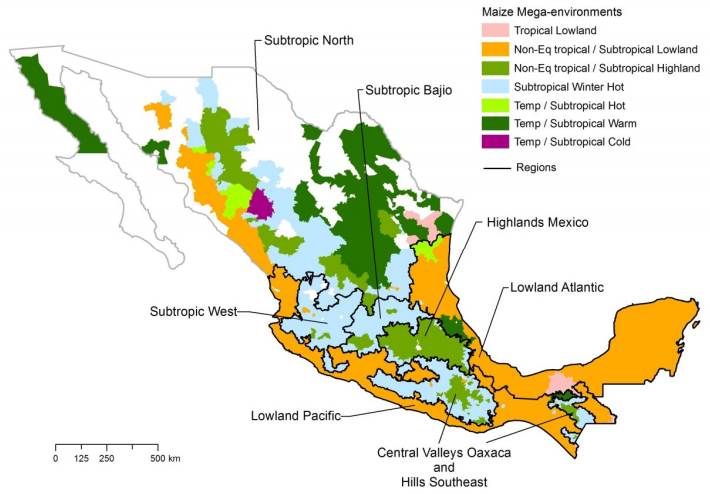
[16] | Hartkamp AD, White JW, Rodríguez Aguilar A, et al. (2000) Maize Production Environments Revisited: A GIS-based Approach. CIMMYT, Mexico D.F. |
[17] | Fischer R, Byerlee D, Edmeades G (2014) Crop yields and global food security: will yield increase continue to feed the world? Canberra: Australian Centre for International Agricultural Research. |
[18] | SIAP, Sistema de Información Agrícola y Pecuaria. Anuario Estadístico de la Producción Agrícola 2012. 2013, Available from: http://infosiap.siap.gob.mx/aagricola_siap/icultivo/index.jsp |
[19] | SIAP, Sistema de Información Agrícola y Pecuaria. Anuario Estadístico de la Producción Agrícola 2012 - 2015. 2016, Available from: http://infosiap.siap.gob.mx/aagricola_siap/icultivo/index.jsp |
[20] | INEGI, Instituto Nacional de Estadística y Geografía. Continuo de Elevaciones Mexicano 2.0. Marco Geoestadístico Nacional MGM. 2014, Available from: http://www.inegi.org.mx/geo/contenidos/datosrelieve/continental/continuoelevaciones.aspx |
[21] | SMN, Servicio Meteorológico Nacional (2015) Resúmenes Mensuales de Temperaturas y Lluvia. |
[22] |
Aigner D, Lovell C, Schmidt P (1977) Formulation and estimation of stochastic frontier production function models. J Econom 6:21-37. doi: 10.1016/0304-4076(77)90052-5
![]() |
[23] |
Battese GE (1992) Frontier production functions and technical efficiency: a survey of empirical applications in agricultural economics. Agric Econ 7: 185-208. doi: 10.1016/0169-5150(92)90049-5
![]() |
[24] | Greene WH (2008) The Econometric Approach to Efficiency Analysis. In: The Measurement of Productive Efficiency and Productivity Change. Oxford University Press. |
[25] | Namonje-Kapembwa T, Black R, Jayne TS (2015) Does Late Delivery of Subsidized Fertilizer Affect Smallholder Maize Productivity and Production? 2015 AAEA & WAEA Joint Annual Meeting, July 26-28, San Francisco, California 205288, Agricultural and Applied Economics Association; Western Agricultural Economics Association. |
[26] | Dadzie S, Dasmani I (2010) Gender difference and farm level efficiency: Meta-frontier production function approach. J Dev Agric Econ 2: 441-451. |
[27] | Hayami Y, Ruttan V (1970) Agricultural productivity differences among countries. Am Econ Rev 60: 895-911. |
[28] | Mehrabi Boshrabadi H, Villano R, Fleming E (2008) Technical efficiency and environmental - technological gaps in wheat production in Kerman Province of Iran: A meta-frontier analysis. Agric Econ 38: 67-76. |
[29] |
Mariano M, Villano R, Fleming E (2011) Technical efficiency of rice farms in different agroclimatic zones in the Philippines: An application of a stochastic metafrontier model. Asian Econ J 25: 245-269. doi: 10.1111/j.1467-8381.2011.02060.x
![]() |
[30] |
Bravo-Ureta B, Greene W, Solis D (2012) Technical Efficiency Analysis Correcting for the Biases from Observed and Unobserved Variables: An Application to a Natural Resource Management Project. Empir Econ 43: 55-72. doi: 10.1007/s00181-011-0491-y
![]() |
[31] | Kunbhaker S, Wang H, Horncastle A (2015) A Practitioner's Guide to Stochastic Frontier Analysis Using Stata, Cambridge University Press. |
1. | Edward L. Kick, Kelly Zering, John Classen, Approaches to agricultural innovation and their effectiveness, 2017, 2, 2471-2086, 370, 10.3934/agrfood.2017.4.370 | |
2. | Aleksandra Król, Jerzy Księżak, Elżbieta Kubińska, Stelios Rozakis, Evaluation of Sustainability of Maize Cultivation in Poland. A Prospect Theory—PROMETHEE Approach, 2018, 10, 2071-1050, 4263, 10.3390/su10114263 | |
3. | Daniela Figueroa, J. Mauricio Galeana-Pizaña, Juan Manuel Núñez, Carlos Anzaldo Gómez, J. Roberto Hernández-Castro, María del Mar Sánchez-Ramírez, Andrea Garduño, Assessing drivers and deterrents of deforestation in Mexico through a public policy tool. The adequacy of the index of economic pressure for deforestation, 2021, 133, 13899341, 102608, 10.1016/j.forpol.2021.102608 | |
4. | Ivania Cerón-Souza, Carlos H. Galeano, Katherine Tehelen, Hugo R. Jiménez, Carolina González, Opportunities and Challenges to Improve a Public Research Program in Plant Breeding and Enhance Underutilized Plant Genetic Resources in the Tropics, 2021, 12, 2073-4425, 1584, 10.3390/genes12101584 | |
5. | Alberto Santillán-Fernández, Yolanda Salinas-Moreno, José René Valdez-Lazalde, Mauricio Antonio Carmona-Arellano, Javier Enrique Vera-López, Santiago Pereira-Lorenzo, Relationship between Maize Seed Productivity in Mexico between 1983 and 2018 with the Adoption of Genetically Modified Maize and the Resilience of Local Races, 2021, 11, 2077-0472, 737, 10.3390/agriculture11080737 | |
6. | Federico García Suárez, Gabriela Pérez Quesada, Los sistemas de gestión predial: diferencias en eficiencia técnica y brechas tecnológicas en los tambos de Uruguay, 2021, 36, 2525-1295, 91, 10.52292/j.estudecon.2019.1661 | |
7. | Jorge Luis González-Cruz, Juan Manuel Torres-Rojo, Diferencias regionales en la producción de maíz blanco de temporal en México, 2024, 15, 2007-9230, e3170, 10.29312/remexca.v15i1.3170 | |
8. | Evans Brako Ntiamoah, Martinson Ankrah Twumasi, Bismark Ameyaw, Edmond Yeboah Nyamah, Dongmei Li, Exploring the impact of agricultural innovation practices on technical efficiency: The case of smallholder pineapple farmers in Ghana, 2024, 1573-2975, 10.1007/s10668-024-04775-3 | |
9. | Venancio Cuevas-Reyes, Jos´é Luis Jolalpa-Barrera, Blanca I. Sánchez-Toledano, Mercedes Borja-Bravo, Pedro Cadena-Iñiguez, Impacto económico del uso de innovaciones agroecológicas en pequeños productores de maíz de Tlaxcala y Oaxaca, 2025, 16, 2007-9230, e3408, 10.29312/remexca.v16i2.3408 | |
10. | Shahin Rasooli, Pabel Antonio Cervantes-Avilés, Mexitli Sandoval-Reyes, Carlos Alberto Huerta-Aguilar, The Mexican maize panorama: Socio-economic study of agricultural productivity and import dependency, 2025, 0030-7270, 10.1177/00307270251343098 |
Region | Mean yield (kg/ha) | Maize area (ha) | Mean altitude (masl) | Mean temperature (℃) | Mean rainfall Apr/Sep (mm) | Mean rainfall Oct/Mar (mm) |
Highlands Mexico | 2467 | 1, 203, 903 | 2154 | 15.9 | 787 | 389 |
Central Valleys Oaxaca and Hills Southeast | 1419 | 908, 459 | 1651 | 19.4 | 867 | 418 |
Subtropic North | 969 | 681, 965 | 1104 | 19.7 | 381 | 221 |
Subtropic West | 5701 | 617, 435 | 1524 | 19.8 | 708 | 264 |
Subtropic Bajio | 2205 | 442, 730 | 1826 | 18.3 | 645 | 288 |
Lowlands Pacific | 2228 | 1, 090, 052 | 653 | 24 | 1188 | 609 |
Lowlands Atlantic | 1831 | 1, 158, 477 | 188 | 25 | 1016 | 759 |
Source: Production data from SIAP [19], averages 2012–2015. Climatic data elaborated by CIMMYT, GIS Lab from INEGI [20], averages 1951–2010. |
1 Highlands Mexico | 2 Central Valleys Oaxaca | 3 Subtropic North | 4 Subtropic West | 5 Subtropic Bajio | 6 Lowland Pacific | 7 Lowland Atlantic | Pooled (all data) | |
Number of observations | 1135 | 722 | 422 | 584 | 218 | 957 | 441 | 4479 |
Maize yield (kg/ha) | 3465 | 3015 | 1631 | 8593 | 3570 | 4030 | 3062 | 3974 |
Seeding rate (1, 000 seeds/ha) | 73.5 | 61.1 | 56.1 | 87.1 | 73.0 | 61.8 | 59.6 | 67.7 |
Farmers using nitrogen | 93% | 93% | 43% | 90% | 79% | 90% | 72% | 85% |
Nitrogen quantity (kg/ha) | 90.9 | 67.9 | 38.5 | 193.4 | 93.6 | 96.5 | 60.8 | 97.1 |
Farmers using potassium | 32% | 10% | 1% | 65% | 14% | 18% | 15% | 24% |
Potassium quantity (kg/ha) | 30.6 | 36.8 | 10.2 | 50.5 | 27.5 | 37.9 | 29.1 | 38.8 |
Farmers using insecticide | 22% | 53% | 27% | 74% | 53% | 71% | 67% | 51% |
Insecticide quantity (l/ha) | 2.1 | 2.7 | 1.0 | 3.3 | 1.2 | 2.6 | 2.4 | 2.5 |
Rainfall during crop (mm) | 670 | 956 | 491 | 743 | 561 | 1064 | 1126 | 833 |
Altitude (masl) | 2380 | 1445 | 1895 | 1483 | 1869 | 530 | 241 | 1436 |
Soil depth: less than 30 cm | 37% | 68% | 33% | 27% | 25% | 57% | 54% | 46% |
Soil depth: more than 30 cm | 63% | 32% | 67% | 73% | 75% | 43% | 46% | 54% |
Erosion: no-low | 73% | 61% | 79% | 85% | 74% | 74% | 76% | 74% |
Erosion: intermediate-high | 27% | 39% | 21% | 15% | 26% | 26% | 24% | 26% |
Crop affected by severe climate: no | 41% | 37% | 44% | 38% | 36% | 47% | 57% | 43% |
Crop affected by severe climate: yes | 59% | 63% | 56% | 62% | 64% | 53% | 43% | 57% |
Crop year: 2012 | 63% | 35% | 58% | 44% | 53% | 46% | 64% | 51% |
Crop year: 2013 | 20% | 28% | 31% | 40% | 12% | 27% | 22% | 26% |
Crop year: 2014 | 9% | 21% | 2% | 5% | 15% | 15% | 5% | 11% |
Crop year: 2015 | 8% | 15% | 9% | 11% | 20% | 12% | 9% | 11% |
Tillage: conventional | 86% | 64% | 91% | 72% | 57% | 59% | 51% | 70% |
Tillage: minimum | 8% | 21% | 6% | 16% | 21% | 27% | 36% | 18% |
Tillage: conservation | 6% | 16% | 3% | 13% | 22% | 14% | 13% | 11% |
Seed: farmer own kept seed | 65% | 55% | 67% | 6% | 36% | 32% | 34% | 45% |
Seed: commercial hybrid | 33% | 24% | 9% | 92% | 35% | 57% | 51% | 44% |
Seed: commercial open pollinated variety | 1% | 20% | 24% | 3% | 29% | 11% | 14% | 11% |
Weeding: none | 8% | 6% | 15% | 17% | 12% | 6% | 9% | 9% |
Weeding: mechanical | 38% | 27% | 48% | 2% | 17% | 9% | 18% | 23% |
Weeding: chemical | 19% | 48% | 8% | 70% | 35% | 73% | 59% | 46% |
Weeding: both mechanical and chemical | 35% | 19% | 29% | 11% | 36% | 13% | 14% | 22% |
Grain use: self-consumption | 32% | 56% | 49% | 3% | 31% | 21% | 20% | 30% |
Grain use: market | 24% | 10% | 11% | 90% | 34% | 26% | 37% | 31% |
Grain use: both self-consumption and market | 45% | 34% | 41% | 8% | 35% | 53% | 43% | 39% |
Farmer schooling: none | 11% | 22% | 11% | 4% | 25% | 17% | 12% | 14% |
Farmer schooling: primary school | 74% | 74% | 82% | 65% | 56% | 69% | 81% | 72% |
Farmer schooling: secondary school and higher education | 14% | 4% | 7% | 32% | 19% | 14% | 7% | 13% |
Management level: low | 30% | 69% | 59% | 8% | 49% | 52% | 58% | 45% |
Management level: high | 69% | 31% | 41% | 92% | 51% | 49% | 42% | 55% |
Variables | Notation | Description |
Output | ||
Log of maize yield | in kg/ha | |
Frontier variables | ||
Input quantities | ||
Log of seed quantity | X1 | in 1, 000 seeds |
Log of nitrogen quantity | X2 | in kg/ha |
Practices | ||
Seed | D1 | 0 farmers own seed |
1 hybrid | ||
2 OPV | ||
Tillage | D2 | 0 conventional |
1 minimum | ||
2 conservation | ||
Grain use | D3 | 0 if all produce is for self-consumption |
1 if all produce is sold to market | ||
2 both | ||
Inefficiency variables | ||
Endowments | ||
Rainfall during crop | U1 | in millimeters |
Top-soil depth > 30 cm | U2 | 0 if soil is shallower than 30 cm |
1 if soil is deeper than 30 cm | ||
Soil erosion | U3 | 0 if soil has moderate or high soil erosion |
1 if soil has no or little soil erosion | ||
Crop affected by severe climate | U4 | 0 if the crop was not affected by severe climate phenomena |
1 if the crop was affected by severe climate phenomenon | ||
Management capacity | ||
Management level | U5 | 0 if farmer considers her ability or expertise in using modern inputs, practices and information of a rather low level relative to other farmers in the area |
1 if farmer considers her ability or expertise in using modern inputs, practices and information of a rather high level relative to other farmers in the area |
Variable | 1 Highlands Mexico | 2 Central Valleys Oaxaca | 3 Subtropic North | 4 Subtropic West | 5 Subtropic Bajio | 6 Lowland Pacific | 7 Lowland Atlantic | Pooled |
Frontier | ||||||||
Seeding rate (1000 seeds/ha) | 0.1836*** | 0.2901*** | 0.1240 | 0.7947*** | 0.4880*** | -0.3602*** | 0.3531*** | 0.6644*** |
0.0649 | 0.0747 | 0.1087 | 0.0823 | 0.1446 | 0.0815 | 0.1025 | 0.0315 | |
Nitrogen quantity (kg/ha) | 0.0265*** | 0.1052*** | 0.0640*** | 0.0167** | 0.0429*** | 0.0359*** | 0.0324*** | 0.0722*** |
0.0085 | 0.0125 | 0.0139 | 0.0073 | 0.0163 | 0.0073 | 0.0115 | 0.0042 | |
Tillage: minimum | 0.1122*** | 0.0653 | -0.2551** | 0.0336 | 0.0651 | 0.0567** | 0.0659 | 0.0541*** |
0.0414 | 0.0426 | 0.1046 | 0.0334 | 0.0648 | 0.0255 | 0.0418 | 0.0173 | |
Tillage: conservation | 0.0995** | 0.1343*** | -0.0642 | -0.0120 | 0.2775*** | 0.0158 | 0.0217 | 0.0519** |
0.0490 | 0.0466 | 0.1598 | 0.0360 | 0.0717 | 0.0327 | 0.0558 | 0.0216 | |
Seed: commercial hybrid | 0.3630*** | 0.5508*** | 0.3332*** | 0.1926*** | 0.2491*** | 0.5187*** | 0.3813*** | 0.4621*** |
0.0259 | 0.0450 | 0.0876 | 0.0617 | 0.0745 | 0.0285 | 0.0476 | 0.0168 | |
Seed: commercial open pollinated variety | -0.0387 | 0.5263*** | 0.2578*** | 0.1611* | 0.3031*** | 0.4013*** | 0.0330 | 0.2595*** |
0.0947 | 0.0451 | 0.0602 | 0.0935 | 0.0683 | 0.0393 | 0.0614 | 0.0225 | |
Grain use: market | 0.3010*** | 0.3055*** | 0.6047*** | 0.3182*** | 0.4114*** | 0.1843*** | 0.3987*** | 0.4336*** |
0.0317 | 0.0594 | 0.0872 | 0.0876 | 0.0797 | 0.0357 | 0.0602 | 0.0212 | |
Grain use: both market and self-consumption | 0.2608*** | 0.2820*** | 0.2155*** | 0.1268 | 0.1641** | 0.1388*** | 0.3490*** | 0.2602*** |
0.0260 | 0.0394 | 0.0511 | 0.0895 | 0.0744 | 0.0307 | 0.0542 | 0.0181 | |
Crop year: 2013 | 0.0822*** | -0.0793* | -0.0287 | 0.1453*** | 0.4229*** | 0.0920*** | 0.0318 | 0.0725*** |
0.0275 | 0.0419 | 0.0542 | 0.0273 | 0.0925 | 0.0269 | 0.0477 | 0.0161 | |
Crop year: 2014 | -0.0670 | -0.0030 | 0.5794*** | 0.0438 | 0.1272 | -0.0206 | -0.0186 | 0.0163 |
0.0412 | 0.0460 | 0.1829 | 0.0542 | 0.0942 | 0.0328 | 0.0810 | 0.0226 | |
Crop year: 2015 | -0.0850** | -0.0585 | 0.5690*** | -0.1125*** | -0.1388* | -0.0356 | -0.2584*** | -0.0468** |
0.0426 | 0.0546 | 0.0868 | 0.0406 | 0.0811 | 0.0365 | 0.0616 | 0.0227 | |
Constant | 7.2182*** | 6.1066*** | 6.5072*** | 4.8611*** | 5.5610*** | 9.4036*** | 5.9762*** | 4.7123*** |
0.2800 | 0.3029 | 0.4285 | 0.3499 | 0.5990 | 0.3339 | 0.4079 | 0.1404 | |
Usigma | ||||||||
Rainfall during crop | -0.2593 | 0.3561 | -3.6397*** | -8.6713 | -7.9071*** | -0.6019** | -1.3989 | -3.1144*** |
0.1757 | 0.4897 | 1.0321 | 15.1222 | 1.7615 | 0.2496 | 0.9390 | 0.7948 | |
Soil depth: more than 30 cm | 0.1302 | -0.7390** | -0.4591 | -32.2183 | -0.5019 | 0.2836** | 0.9451 | -0.2494* |
0.1147 | 0.3422 | 0.5237 | 2, 821.7 | 0.4301 | 0.1230 | 0.6812 | 0.1516 | |
Erosion: no–low | -0.5144*** | 0.0156 | -1.4175*** | -0.6350 | -1.0351** | -0.2737** | 0.1562 | -0.5711*** |
0.1185 | 0.2661 | 0.5074 | 4.6970 | 0.4504 | 0.1328 | 0.8829 | 0.1695 | |
Crop affected by severe climate: yes | 0.5696*** | 2.9722** | 2.1534** | -43.7234 | -0.4918 | 0.3894*** | 27.8370 | 1.0203*** |
0.1149 | 1.3440 | 0.9047 | 20, 618.9 | 0.4198 | 0.1282 | 1104.7 | 0.1688 | |
Management level: high | -0.2215* | -0.7175** | 0.5956 | 34.5014 | -0.6963 | -0.4367*** | 1.3086** | -0.6507*** |
0.1325 | 0.3634 | 0.4748 | 99.0008 | 0.4420 | 0.1289 | 0.6415 | 0.1296 | |
Constant | 0.3168 | -6.8294* | 18.8427*** | 17.2035 | 48.9434*** | 2.6157 | -22.2181 | 17.6971*** |
1.1773 | 4.1044 | 6.0750 | 11.0060 | 1.7394 | 1104.8 | 4.7550 | ||
Vsigma | ||||||||
Constant | -2.9012*** | -1.8750*** | -1.6212*** | -2.5750*** | -2.3171*** | -3.0665*** | -2.1688*** | -1.7879*** |
0.1256 | 0.0985 | 0.0827 | 0.0585 | 0.1580 | 0.1451 | 0.0770 | 0.0531 | |
E (sigma_u) | 0.4902 | 0.2874 | 0.2271 | 0.0031 | 0.4064 | 0.4456 | 0.1248 | 0.2328 |
sigma_v | 0.2344*** | 0.3916*** | 0.4446*** | 0.2760*** | 0.3139*** | 0.2158*** | 0.3381*** | 0.4090*** |
0.0147 | 0.0193 | 0.0184 | 0.0081 | 0.0248 | 0.0157 | 0.0130 | 0.0109 | |
Wald chi2(11) | 546.8 | 675.4 | 223.6 | 400.5 | 236.0 | 520.5 | 444.1 | 4576.8 |
Prob > chi2 | 0.0000 | 0.0000 | 0.0000 | 0.0000 | 0.0000 | 0.0000 | 0.0000 | 0.0000 |
Log likelihood | -476.0 | -421.5 | -280.8 | -76.8 | -102.4 | -319.0 | -173.9 | -2660.1 |
Number of observations | 1135 | 722 | 422 | 584 | 218 | 957 | 441 | 4479 |
Statistical significance: *** = 1%, ** = 5%, * = 10% |
Variable | Pooled | Metafrontier |
Seeding rate (1000 seeds/ha) | 0.6644*** | 0.1138 |
Nitrogen quantity (kg/ha) | 0.0722*** | 0.0221 |
Tillage: minimum | 0.0541*** | 0.0563 |
Tillage: conservation | 0.0519** | 0.0585 |
Seed: hybrid | 0.4621*** | 0.2321 |
Seed: OPV | 0.2595*** | 0.0515 |
Grain use: market | 0.4336*** | 0.4883 |
Grain use: both | 0.2602*** | 0.1596 |
Year: 2013 | 0.0725*** | 0.1469 |
Year: 2014 | 0.0163 | 0.0058 |
Year: 2015 | -0.0468** | -0.0841 |
Constant | 4.7123*** | 7.8666 |
Statistical significance: *** = 1%, ** = 5%, * = 10% |
Region | Technical efficiency (TE) | Metatechnology ratio (MTR) | Total efficiency (Tem) | Maize productivity (kg/ha) |
1 Highlands Mexico | 70% | 75% | 52% | 3465 |
2 Central Valleys Oaxaca | 81% | 59% | 47% | 3015 |
3 Subtropic North | 84% | 32% | 27% | 1631 |
4 Subtropic West | 100% | 82% | 82% | 8593 |
5 Subtropic Bajio | 78% | 62% | 48% | 3570 |
6 Lowland Pacific | 72% | 78% | 56% | 4030 |
7 Lowland Atlantic | 92% | 45% | 42% | 3062 |
Region | Farmers in MasAgro | Average farmers | Difference (%) |
1 Highlands Mexico | 3465 | 2467 | 40 |
2 Central Valleys Oaxaca | 3015 | 1419 | 112 |
3 Subtropic North | 1631 | 969 | 68 |
4 Subtropic West | 8593 | 5701 | 51 |
5 Subtropic Bajio | 3570 | 2205 | 62 |
6 Lowland Pacific | 4030 | 2228 | 81 |
7 Lowland Atlantic | 3062 | 1831 | 67 |