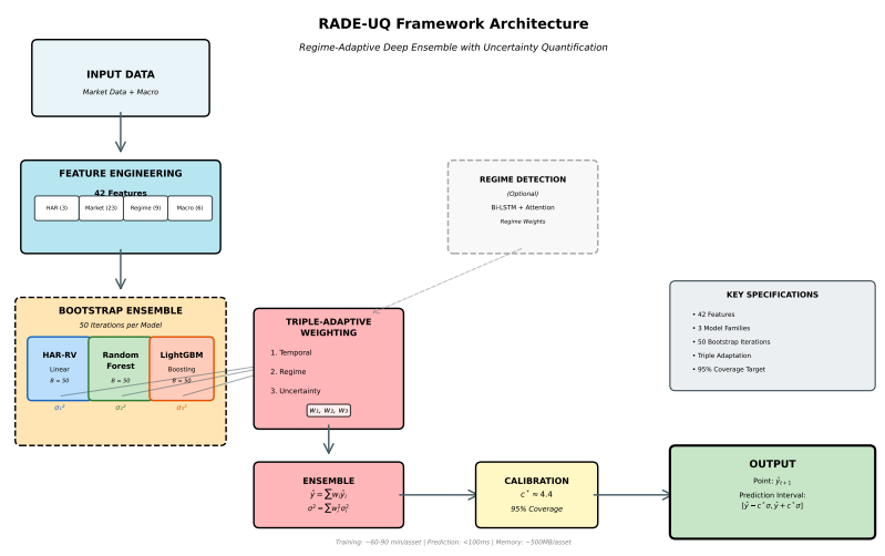
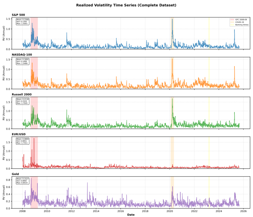
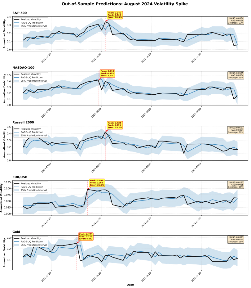
Accurate volatility forecasting, which is critical for financial risk management, has been challenged by classic econometric models and recent machine learning algorithms that lack reliable uncertainty quantification. The regime-adaptive deep ensemble with uncertainty quantification solution combines bidirectional long short-term memory (Bi-LSTM) for regime identification and bootstrap uncertainty quantification with models such as the heterogeneous autoregressive model for realized volatility (HAR-RV), random forest, and light gradient-boosting machine (LightGBM). It also includes triple-adaptive ensemble weighting. A 10-year investigation of S&P 500 data showed a 55.6% improvement in RMSE compared to the heterogeneous autoregressive model for realized volatility (HAR-RV) baseline and an $ R^2 $ increase from 0.602 to 0.922. The approach demonstrated confirmed 95% prediction intervals, outstanding adaptability, and performance across several regimes. Cross-asset validation across five asset classes (S&P 500, NASDAQ-100, Russell 2000, EUR/USD, and Gold) confirms consistent root mean square error (RMSE) improvements of 47–55% over HAR-RV and $ R^2 $ above 0.89 across all assets, demonstrating robust generalizability. Economic evaluations show a 94.6% reduction in portfolio volatility and an enhanced Sharpe ratio. This framework outperforms previous methods by providing high accuracy, well-calibrated uncertainty estimates, and a thorough economic analysis.
Citation: Khalid Jeaab, Smaaine Ouaharahe, Youness Saoudi. Uncertainty calibrated volatility forecasting through regime detection and adaptive ensemble modeling[J]. Data Science in Finance and Economics, 2026, 6(3): 475-507. doi: 10.3934/DSFE.2026017
Accurate volatility forecasting, which is critical for financial risk management, has been challenged by classic econometric models and recent machine learning algorithms that lack reliable uncertainty quantification. The regime-adaptive deep ensemble with uncertainty quantification solution combines bidirectional long short-term memory (Bi-LSTM) for regime identification and bootstrap uncertainty quantification with models such as the heterogeneous autoregressive model for realized volatility (HAR-RV), random forest, and light gradient-boosting machine (LightGBM). It also includes triple-adaptive ensemble weighting. A 10-year investigation of S&P 500 data showed a 55.6% improvement in RMSE compared to the heterogeneous autoregressive model for realized volatility (HAR-RV) baseline and an $ R^2 $ increase from 0.602 to 0.922. The approach demonstrated confirmed 95% prediction intervals, outstanding adaptability, and performance across several regimes. Cross-asset validation across five asset classes (S&P 500, NASDAQ-100, Russell 2000, EUR/USD, and Gold) confirms consistent root mean square error (RMSE) improvements of 47–55% over HAR-RV and $ R^2 $ above 0.89 across all assets, demonstrating robust generalizability. Economic evaluations show a 94.6% reduction in portfolio volatility and an enhanced Sharpe ratio. This framework outperforms previous methods by providing high accuracy, well-calibrated uncertainty estimates, and a thorough economic analysis.

| [1] |
Andersen TG, Bollerslev T, Diebold FX, et al. (2001) The distribution of realized stock return volatility. J Financ Econ 61: 43–76. https://doi.org/10.1016/S0304-405X(01)00055-1 doi: 10.1016/S0304-405X(01)00055-1

|
| [2] |
Andersen TG, Bollerslev T, Diebold FX, et al. (2003) Modeling and forecasting realized volatility. Econometrica 71: 579–625. https://doi.org/10.1111/1468-0262.00418 doi: 10.1111/1468-0262.00418
|
| [3] | Bahdanau D, Cho K, Bengio Y (2015) Neural machine translation by jointly learning to align and translate. In: International Conference on Learning Representations. |
| [4] |
Barndorff-Nielsen OE, Shephard N (2002) Econometric analysis of realized volatility and its use in estimating stochastic volatility models. J R Stat Soc B 64: 253–280. https://doi.org/10.1111/1467-9868.00336 doi: 10.1111/1467-9868.00336
|
| [5] |
Bollerslev T (1986) Generalized autoregressive conditional heteroskedasticity. J Econometrics 31: 307–327. https://doi.org/10.1016/0304-4076(86)90063-1 doi: 10.1016/0304-4076(86)90063-1
|
| [6] |
Breiman L (1996) Bagging predictors. Mach Learn 24: 123–140. https://doi.org/10.1023/A:1018054314350 doi: 10.1023/A:1018054314350
|
| [7] |
Breiman L (2001) Random forests. Mach Learn 45: 5–32. https://doi.org/10.1023/A:1010933404324 doi: 10.1023/A:1010933404324
|
| [8] | Cho K, Van Merriënboer B, Gulcehre C, et al. (2014) Learning phrase representations using RNN encoder-decoder for statistical machine translation. In: Conference on Empirical Methods in Natural Language Processing, 1724–1734. |
| [9] |
Christensen K, Siggaard M, Veliyev B (2023) A machine learning approach to volatility forecasting. J Financ Econometrics 21: 1680–1727. https://doi.org/10.1093/jjfinec/nbac020 doi: 10.1093/jjfinec/nbac020
|
| [10] |
Christoffersen PF (1998) Evaluating interval forecasts. Int Econ Rev 39: 841–862. https://doi.org/10.2307/2527341 doi: 10.2307/2527341
|
| [11] |
Corsi F (2009) A simple approximate long-memory model of realized volatility. Jo Financ Econometrics 7: 174–196. https://doi.org/10.1093/jjfinec/nbp001 doi: 10.1093/jjfinec/nbp001
|
| [12] | Fleming J, Kirby C, Ostdiek B (2001) The economic value of volatility timing. J Financ 56: 329–352. |
| [13] |
Fleming J, Kirby C, Ostdiek B (2003) The economic value of volatility timing using "realized" volatility. J Financ Econ 67: 473–509. https://doi.org/10.1016/S0304-405X(02)00259-3 doi: 10.1016/S0304-405X(02)00259-3
|
| [14] |
Gneiting T, Raftery AE (2007) Strictly proper scoring rules, prediction, and estimation. J Am Stat Assoc 102: 359–378. https://doi.org/10.1198/016214506000001437 doi: 10.1198/016214506000001437
|
| [15] |
Hamilton JD (1989) A new approach to the economic analysis of nonstationary time series and the business cycle. Econometrica 57: 357–384. https://doi.org/10.2307/1912559 doi: 10.2307/1912559
|
| [16] |
Hansen PR, Lunde A (2005) A forecast comparison of volatility models: Does anything beat a GARCH(1, 1)? J Appl Econometrics 20: 873–889. https://doi.org/10.1002/jae.800 doi: 10.1002/jae.800
|
| [17] |
Hochreiter S, Schmidhuber J (1997) Long short-term memory. Neural Comput 9: 1735–1780. https://doi.org/10.1162/neco.1997.9.8.1735 doi: 10.1162/neco.1997.9.8.1735
|
| [18] | Ke G, Meng Q, Finley T, et al (2017) LightGBM: A highly efficient gradient boosting decision tree. Adv Neur Inf Process Syst 30: 3146–3154. |
| [19] | Kupiec PH (1995) Techniques for verifying the accuracy of risk measurement models. J Deriv 3: 73–84. |
| [20] |
Patton AJ (2011) Volatility forecast comparison using imperfect volatility proxies. J Econometrics 160: 246–256. https://doi.org/10.1016/j.jeconom.2010.03.034 doi: 10.1016/j.jeconom.2010.03.034
|
| [21] | Vaswani A, Shazeer N, Parmar N, et al. (2017) Attention is all you need. Adv Neur Inf Process Syst 30: 5998–6008. |
| [22] | Vovk V, Gammerman A, Shafer G (2005) Algorithmic Learning in a Random World. Springer. |
| [23] |
West KD (1996) Asymptotic inference about predictive ability. Econometrica 64: 1067–1084. https://doi.org/10.2307/2171956 doi: 10.2307/2171956
|
| [24] | Zhou ZH (2012) Ensemble methods: Foundations and algorithms. |
 DSFE-06-03-017-s001.pdf |
 |
Figures(3) / Tables(13)
Khalid Jeaab, Smaaine Ouaharahe, Youness Saoudi. Uncertainty calibrated volatility forecasting through regime detection and adaptive ensemble modeling[J]. Data Science in Finance and Economics, 2026, 6(3): 475-507. doi: 10.3934/DSFE.2026017





 DownLoad: