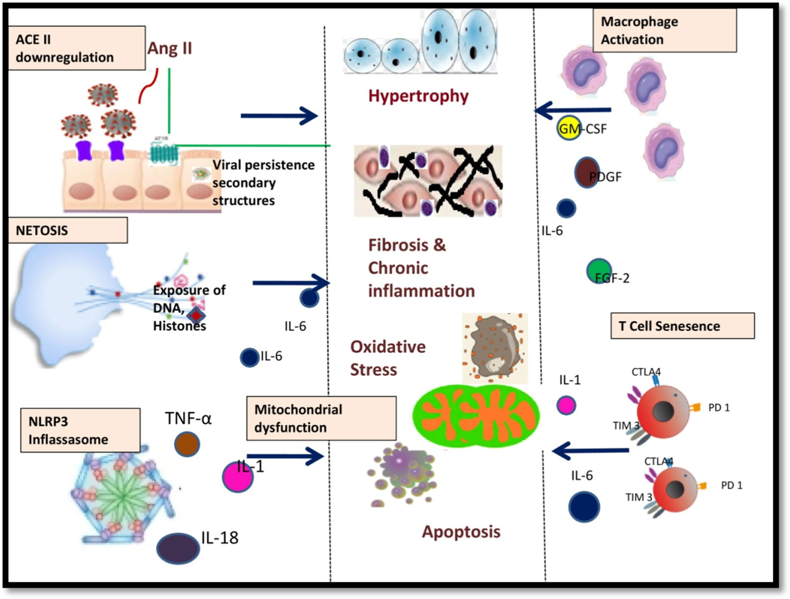
Since the emergence of SARS-COV-2, many updates and assumptions are being discussed based on the emerging understanding of the pathophysiology and outcomes of the infection. The host immune response is the critical factor in disease severity and the unique immune response of each individual has resulted in a broad spectrum of disease severity and clinical presentations. In this article, combining the emerging knowledge on the immunopathogenesis of COVID-19 infection with insights into the underlying mechanisms of certain autoimmune and chronic Immune-mediated inflammatory diseases we propound our hypothesis that SARS-CoV-2 infection produces chronic viral inflammatory syndrome.
Citation: DharmaSaranya Gurusamy, Vasuki Selvamurugesan, Swaminathan Kalyanasundaram, Shantaraman Kalyanaraman. Is COVID 19, a beginning of new entity called chronic viral systemic inflammatory syndrome?[J]. AIMS Allergy and Immunology, 2021, 5(2): 127-134. doi: 10.3934/Allergy.2021010
Since the emergence of SARS-COV-2, many updates and assumptions are being discussed based on the emerging understanding of the pathophysiology and outcomes of the infection. The host immune response is the critical factor in disease severity and the unique immune response of each individual has resulted in a broad spectrum of disease severity and clinical presentations. In this article, combining the emerging knowledge on the immunopathogenesis of COVID-19 infection with insights into the underlying mechanisms of certain autoimmune and chronic Immune-mediated inflammatory diseases we propound our hypothesis that SARS-CoV-2 infection produces chronic viral inflammatory syndrome.
disabled homolog 1
surfeit locus protein 1
apoptosis-inducing factor mitochondrial
T cell immunoglobulin and mucin domain 3
cytotoxic T lymphocyte associated protein 4
programmed cell death protein 1
T cell immunoglobulin and ITIM domain receptor
mitochondrial antiviral signaling proteins
voltage dependent anion channel
angiotensin converting enzyme II
angiotensin I receptor
nuclear NOD, LRR, pyrin domain containing protein 3
interleukin
granulocyte monocyte colony stimulating factor
tumor necrosis factor
platelet derived growth factor
fibroblast growth factor
Interferon gamma
tumor necrosis factor alpha
nuclear factor κB

| [1] |
Ong KC, Ng AWK, Lee LSU, et al. (2004) Pulmonary function and exercise capacity in survivors of severe acute respiratory syndrome. Eur Respir J 24: 436-442. doi: 10.1183/09031936.04.00007104

|
| [2] |
Gombar S, Chang M, Hogan CA, et al. (2020) Persistent detection of SARS-CoV-2 RNA in patients and healthcare workers with COVID-19. J Clin Virol 129: 104477. doi: 10.1016/j.jcv.2020.104477
|
| [3] |
Li N, Wang X, Lv T (2020) Prolonged SARS-CoV-2 RNA shedding: Not a rare phenomenon. J Med Virol 92: 2286-2287. doi: 10.1002/jmv.25952
|
| [4] |
Simmonds P, Tuplin A, Evans DJ (2004) Detection of genome-scale ordered RNA structure (GORS) in genomes of positive-stranded RNA viruses: implications for virus evolution and host persistence. RNA 10: 1337-1351. doi: 10.1261/rna.7640104
|
| [5] |
Lucchese G, Flöel A (2020) Molecular mimicry between SARS-CoV-2 and respiratory pacemaker neurons. Autoimmun Rev 19: 102556. doi: 10.1016/j.autrev.2020.102556
|
| [6] |
Angileri F, Legare S, Gammazza AM, et al. (2020) Molecular mimicry may explain multi-organ damage in COVID-19. Autoimmun Rev 19: 102591. doi: 10.1016/j.autrev.2020.102591
|
| [7] |
Gheblawi M, Wang K, Viveiros A, et al. (2020) Angiotensin-converting enzyme 2: SARS-CoV-2 receptor and regulator of the renin-angiotensin system: celebrating the 20th anniversary of the discovery of ACE2. Circ Res 126: 1456-1474. doi: 10.1161/CIRCRESAHA.120.317015
|
| [8] |
Kamo T, Akazawa H, Komuro I (2015) Pleiotropic effects of angiotensin II receptor signaling in cardiovascular homeostasis and aging. Int Heart J 56: 249-254. doi: 10.1536/ihj.14-429
|
| [9] |
Verdecchia P, Cavallini C, Spanevello A, et al. (2020) The pivotal link between ACE2 deficiency and SARS-CoV-2 infection. Eur J Intern Med 76: 14-20. doi: 10.1016/j.ejim.2020.04.037
|
| [10] |
Tseng YH, Yang RC, Lu TS (2020) Two hits to the renin-angiotensin system may play a key role in severe COVID-19. Kaohsiung J Med Sci 36: 389-392. doi: 10.1002/kjm2.12237
|
| [11] |
Nieto-Torres JL, Verdiá-Báguena C, Jimenez-Guardeño JM, et al. (2015) Severe acute respiratory syndrome coronavirus E protein transports calcium ions and activates the NLRP3 inflammasome. Virology 485: 330-339. doi: 10.1016/j.virol.2015.08.010
|
| [12] |
Hoffman HM, Wanderer AA, Broide DH (2001) Familial cold autoinflammatory syndrome: phenotype and genotype of an autosomal dominant periodic fever. J Allergy Clin Immun 108: 615-620. doi: 10.1067/mai.2001.118790
|
| [13] | Muckle TJ, Wells M (1962) Urticaria, deafness, and amyloidosis: a new heredo-familial syndrome. QJM-Int J Med 31: 235-248. |
| [14] |
Prieur AM, Griscelli C, Lampert F, et al. (1987) A chronic, infantile, neurological, cutaneous and articular (CINCA) syndrome. A specific entity analysed in 30 patients. Scand J Rheumatol 16: 57-68. doi: 10.3109/03009748709102523
|
| [15] |
Wang C, Xie J, Zhao L, et al. (2020) Alveolar macrophage dysfunction and cytokine storm in the pathogenesis of two severe COVID-19 patients. EBioMedicine 57: 102833. doi: 10.1016/j.ebiom.2020.102833
|
| [16] |
Liao M, Liu Y, Yuan J, et al. (2020) Single-cell landscape of bronchoalveolar immune cells in patients with COVID-19. Nat Med 26: 842-844. doi: 10.1038/s41591-020-0901-9
|
| [17] |
Hou J, Shi J, Chen L, et al. (2018) M2 macrophages promote myofibroblast differentiation of LR-MSCs and are associated with pulmonary fibrogenesis. Cell Commun Signaling 16: 89. doi: 10.1186/s12964-018-0300-8
|
| [18] | Zuo Y, Yalavarthi S, Shi H, et al. (2020) Neutrophil extracellular traps (NETs) as markers of disease severity in COVID-19. JCI Insight 5: e138999. |
| [19] |
Gupta S, Kaplan MJ (2016) The role of neutrophils and NETosis in autoimmune and renal diseases. Nat Rev Nephrol 12: 402-413. doi: 10.1038/nrneph.2016.71
|
| [20] |
Diao B, Wang C, Tan Y, et al. (2020) Reduction and functional exhaustion of T cells in patients with coronavirus disease 2019 (COVID-19). Front Immunol 11: 827. doi: 10.3389/fimmu.2020.00827
|
| [21] |
Lopes-Paciencia S, Saint-Germain E, Rowell MC, et al. (2019) The senescence-associated secretory phenotype and its regulation. Cytokine 117: 15-22. doi: 10.1016/j.cyto.2019.01.013
|
| [22] |
Weyand CM, Yang Z, Goronzy JJ (2014) T cell aging in rheumatoid arthritis. Curr Opin Rheumatol 26: 93-100. doi: 10.1097/BOR.0000000000000011
|
| [23] |
Ichinohe T, Yamazaki T, Koshiba T, et al. (2013) Mitochondrial protein mitofusin 2 is required for NLRP3 inflammasome activation after RNA virus infection. P Natl Acad Sci USA 110: 17963-17968. doi: 10.1073/pnas.1312571110
|
| [24] |
Park S, Juliana C, Hong S, et al. (2013) The mitochondrial antiviral protein MAVS associates with NLRP3 and regulates its inflammasome activity. J Immunol 191: 4358-4366. doi: 10.4049/jimmunol.1301170
|
| [25] |
Thompson EA, Cascino K, Ordonez AA, et al. (2021) Metabolic programs define dysfunctional immune responses in severe COVID-19 patients. Cell Rep 34: 108863. doi: 10.1016/j.celrep.2021.108863
|
| [26] |
Kim J, Gupta R, Blanco LP, et al. (2019) VDAC oligomers form mitochondrial pores to release mtDNA fragments and promote lupus-like disease. Science 366: 1531-1536. doi: 10.1126/science.aav4011
|
| [27] |
Camara AKS, Zhou Y, Wen PC, et al. (2017) Mitochondrial VDAC1: a key gatekeeper as potential therapeutic target. Front Physiol 8: 460. doi: 10.3389/fphys.2017.00460
|
| [28] |
Lood C, Blanco LP, Purmalek MM, et al. (2016) Neutrophil extracellular traps enriched in oxidized mitochondrial DNA are interferogenic and contribute to lupus-like disease. Nat Med 22: 146. doi: 10.1038/nm.4027
|
| [29] |
Vernochet C, Kahn CR (2012) Mitochondria, obesity and aging. Aging (Albany NY) 4: 859. doi: 10.18632/aging.100518
|
| [30] |
Hamming I, Timens W, Bulthuis MLC, et al. (2004) Tissue distribution of ACE2 protein, the functional receptor for SARS coronavirus. A first step in understanding SARS pathogenesis. J Pathol 203: 631-637. doi: 10.1002/path.1570
|
| [31] |
Combet M, Pavot A, Savale L, et al. (2020) Rapid onset honeycombing fibrosis in spontaneously breathing patient with Covid-19. Eur Respir J 56: 2001808. doi: 10.1183/13993003.01808-2020
|
| [32] |
Verdoni L, Mazza A, Gervasoni A, et al. (2020) An outbreak of severe Kawasaki-like disease at the Italian epicentre of the SARS-CoV-2 epidemic: an observational cohort study. Lancet 395: 1771-1778. doi: 10.1016/S0140-6736(20)31103-X
|
| [33] | Rajpal S, Tong MS, Borchers J, et al. (2021) Cardiovascular magnetic resonance findings in competitive athletes recovering from COVID-19 infection. JAMA Cardiol 6: 116-118. |
Figures(2) / Tables(1)

DharmaSaranya Gurusamy, Vasuki Selvamurugesan, Swaminathan Kalyanasundaram, Shantaraman Kalyanaraman. Is COVID 19, a beginning of new entity called chronic viral systemic inflammatory syndrome?[J]. AIMS Allergy and Immunology, 2021, 5(2): 127-134. doi: 10.3934/Allergy.2021010


 DownLoad: