The moon lander optimal control problem revisited

Filippo Gazzola; Elsa M. Marchini; Filippo Gazzola; Elsa M. Marchini

doi:10.3934/mine.2021040

Mathematics in Engineering

2021, Volume 3, Issue 5:1-14. doi: 10.3934/mine.2021040

Previous Article Next Article

Research article Special Issues

The moon lander optimal control problem revisited

Filippo Gazzola ^,,
Elsa M. Marchini

Dipartimento di Matematica, Politecnico di Milano, Piazza L. da Vinci, 32 - 20133 Milano, Italy

Received: 16 June 2020 Accepted: 09 September 2020 Published: 13 October 2020

Abstract
Full Text(HTML)
Download PDF

We revisit the control problem for a spacecraft to land on the moon surface at rest with minimal fuel consumption. We show that a detailed analysis in the related 3D phase space uncovers the existence of infinitely many safe landing curves, contrary to several former 2D descriptions that implicitly claim the existence of just one such curve. Our results lead to a deeper understanding of the dynamics and allows for a precise characterization of the optimal control. Such control is known to be bang-bang and our results give a full characterization of the switch position.
- optimal control,
- bang-bang,
- moon lander
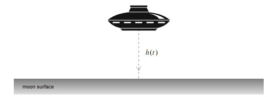
Citation: Filippo Gazzola, Elsa M. Marchini. The moon lander optimal control problem revisited[J]. Mathematics in Engineering, 2021, 3(5): 1-14. doi: 10.3934/mine.2021040

Related Papers:

Abstract

We revisit the control problem for a spacecraft to land on the moon surface at rest with minimal fuel consumption. We show that a detailed analysis in the related 3D phase space uncovers the existence of infinitely many safe landing curves, contrary to several former 2D descriptions that implicitly claim the existence of just one such curve. Our results lead to a deeper understanding of the dynamics and allows for a precise characterization of the optimal control. Such control is known to be bang-bang and our results give a full characterization of the switch position.

References

[1]	Evans LC, An Introduction to Mathematical Optimal Control Theory. Available from: https://math.berkeley.edu/evans/control.course.pdf.
[2]	Fattorini HO (1999) Infinite-Dimensional Optimization and Control Theory, Cambridge: Cambridge University Press.
[3]	Fleming W, Rishel R (1975) Deterministic and Stochastic Optimal Control, Springer.
[4]	Meditch JS (1964) On the problem of optimal thrust programming for a lunar soft kanding. IEEE T Automat Contr 9: 477–484.
[5]	Miele A (1962) The calculus of variations in applied aerodynamics and flight mechanics, In: Optimization Techniques with Applications to Aerospace Systems, Academic Press, 99–170.

Reader Comments

your name:*

Email:*
© 2021 the Author(s), licensee AIMS Press. This is an open access article distributed under the terms of the Creative Commons Attribution License (http://creativecommons.org/licenses/by/4.0)