Open Access Journals

AIMS Microbiology, 2018, 4(2): 261-273. doi: 10.3934/microbiol.2018.2.261. Review Topical Section

Export file:

Format

RIS(for EndNote,Reference Manager,ProCite)
BibTex
Text

Content

Citation Only
Citation and Abstract

Industrial production, application, microbial biosynthesis and degradation of furanic compound, hydroxymethylfurfural (HMF)

Yu Wang, Caroline A. Brown, Rachel Chen

1 Department of Chemistry and Biochemistry, University of North Georgia-Dahlonega, Dahlonega, GA, 30597, USA
2 School of Chemical & Biomolecular Engineering, Georgia Institute of Technology, Atlanta, GA 30332, USA

Received: , Accepted: , Published:

Topical Section: Microbial physiology and metabolism

Abstract Full Text(HTML) Figure/Table

Biorefinery is increasingly embraced as an environmentally friendly approach that has the potential to shift current petroleum-based chemical and material manufacture to renewable sources. Furanic compounds, particularly hydroxymethylfurfurals (HMFs) are platform chemicals, from which a variety of value-added chemicals can be derived. Their biomanufacture and biodegradation therefore will have a large impact. Here, we first review the potential industrial production of 4-HMF and 5-HMF, then we summarize the known microbial biosynthesis and biodegradation pathways of furanic compounds with emphasis on the enzymes in each pathway. We especially focus on the structure, function and catalytic mechanism of MfnB (4-(hydroxymethyl)-2-furancarboxyaldehyde-phosphate synthase) and hmfH (HMF oxidase), which catalyze the formation of phosphorylated 4-HMF and the oxidation of 5-HMF to furandicarboxylic acid (2,5-FDCA), respectively. Understanding the structure-function relationship of these enzymes will provide important insights in enzyme engineering, which eventually will find industry applications in mass-production of biobased polymers and other bulk chemicals in future.

Figure/Table

Supplementary

Article Metrics

Keywords: furan-containing compound; 4-HMF; 5-HMF; HMF metabolism; HMF biosynthesis; HMF degradation

Citation: Yu Wang, Caroline A. Brown, Rachel Chen. Industrial production, application, microbial biosynthesis and degradation of furanic compound, hydroxymethylfurfural (HMF). AIMS Microbiology, 2018, 4(2): 261-273. doi: 10.3934/microbiol.2018.2.261

References:

1. Bozell JJ, Petersen GR (2010) Technology development for the production of biobased products from biorefinery carbohydrates-the US Department of Energy's "Top 10" revisited. Green Chem 12: 539–517.
2. Werpy T, Petersen G (2004) Top Value Added Chemicals from Biomass, National Renewable Energy Laboratory: Golden, CO.
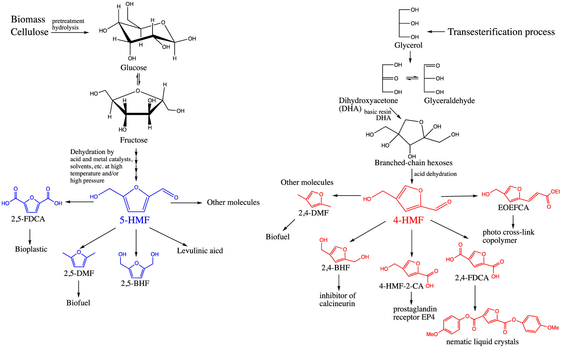
3. Zhang D, Dumont MJ (2017) Advances in polymer precursors and bio-based polymers synthesized from 5-hydroxymethylfurfural. J Polym Sci Pol Chem 55: 1478–1492.
4. Deng J, Pan T, Xu Q, et al. (2013) Linked strategy for the production of fuels via formose reaction. Sci Rep 3: 1244.
5. Rosatella AA, Simeonov SP, Frade RFM, et al. (2011) 5-Hydroxymethylfurfural (HMF) as a building block platform: Biological properties, synthesis and synthetic applications. Green Chem 13: 754–741.
6. Cui MS, Deng J, Li XL, et al. (2016) Production of 4-Hydroxymethylfurfural from derivatives of biomass-derived glycerol for chemicals and polymers. ACS Sustain Chem Eng 4: 1707–1714.
7. van Putten RJ, van der Waal JC, de Jong ED, et al. (2013) Hydroxymethylfurfural, a versatile platform chemical made from renewable resources. Chem Rev 113: 1499–1597.
8. Yu IKM, Tsang DCW (2017) Conversion of biomass to hydroxymethylfurfural: A review of catalytic systems and underlying mechanisms. Bioresource Technol 238: 716–732.
9. Qin YZ, Zong MH, Lou WY, et al. (2016) Biocatalytic upgrading of 5-Hydroxymethylfurfural (HMF) with levulinic acid to HMF levulinate in biomass-derived solvents. ACS Sustain Chem Eng 4: 4050–4054.
10. Bohre A, Dutta S, Saha B, et al. (2015) Upgrading furfurals to drop-in biofuels: An overview. ACS Sustain Chem Eng 3: 1263–1277.
11. Caes BR, Teixeira RE, Knapp KG, et al. (2015) Biomass to furanics: Renewable routes to chemicals and fuels. ACS Sustain Chem Eng 3: 2591–2605.
12. Alexandrino K, Millera Á, Bilbao R, et al. (2014) Interaction between 2,5-dimethylfuran and nitric oxide: Experimental and modeling study. Energ Fuel 28: 4193–4198.
13. Zhong S, Daniel R, Xu H, et al. (2010) Combustion and emissions of 2,5-dimethylfuran in a direct-injection spark-ignition engine. Energ Fuel 24: 2891–2899.
14. Ray P, Smith C, Simon G, et al. (2017) Renewable green platform chemicals for polymers. Molecules 12: 376.
15. Burgess SK, Leisen JE, Kraftschik BE, et al. (2014) Chain mobility, thermal, and mechanical properties of poly(ethylene furanoate) compared to poly(ethylene terephthalate). Macromolecules 47: 1383–1391.
16. Papageorgiou GZ, Tsanaktsis V, Bikiaris DN (2014) Synthesis of poly(ethylene furandicarboxylate) polyester using monomers derived from renewable resources: thermal behavior comparison with PET and PEN. Phys Chem Chem Phys 16: 7946–7958.
17. Codou A, Moncel M, van Berkel JG, et al. (2016) Glass transition dynamics and cooperativity length of poly(ethylene 2,5-furandicarboxylate) compared to poly(ethylene terephthalate). Phys Chem Chem Phys 18: 16647–16658.
18. Dimitriadis T, Bikiaris DN, Papageorgiou GZ, et al. (2016) Molecular dynamics of poly(ethylene-2,5-furanoate) (PEF) as a function of the degree of crystallinity by dielectric spectroscopy and calorimetry. Macromol Chem Phys 217: 2056–2062.
19. Lomelí-Rodríguez M, Martín-Molina M, Jiménez-Pardo M, et al. (2016) Synthesis and kinetic modeling of biomass-derived renewable polyesters. J Polym Sci Pol Chem 54: 2876–2887.
20. Terzopoulou Z, Tsanaktsis V, Nerantzaki M, et al. (2016) Thermal degradation of biobased polyesters: Kinetics and decomposition mechanism of polyesters from 2,5-furandicarboxylic acid and long-chain aliphatic diols. J Anal Appl Pyrol 117: 162–175.
21. Baba Y, Hirukawa N, Tanohira N, et al. (2003) Structure-based design of a highly selective catalytic site-directed inhibitor of Ser/Thr protein phosphatase 2B (Calcineurin). J Am Chem Soc 125: 9740–9749.
22. Clark DE, Clark KL, Coleman RA, et al. (2005) Patent No. WO2004067524.
23. Ermakov S, Beletskii A, Eismont O, et al. (2015) Brief review of liquid crystals, In: Liquid Crystals in Biotribology, Springer, 37–56.
24. Dewar MJS, Riddle RM (1975) Factors influencing the stabilities of nematic liquid crystals. J Am Chem Soc 97: 6658–6662.
25. Kowalski S, Lukasiewicz M, Duda-Chodak A, et al. (2013) 5-hydroxymethyl-2-furfural (HMF)-heat-induced formation, occurrence in food and biotransformation-a review. Pol J Food Nutr Sci 63: 207–225.
26. Murkovic M, Bornik MA (2007) Formation of 5-hydroxymethyl-2-furfural (HMF) and 5-hydroxymethyl-2-furoic acid during roasting of coffee. Mol Nutr Food Res 51: 390–394.
27. Murkovic M, Pichler N (2006) Analysis of 5-hydroxymethylfurfual in coffee, dried fruits and urine. Mol Nutr Food Res 50: 842–846.
28. Saha B, Abu-Omar MM (2014) Advances in 5-hydroxymethylfurfural production from biomass in biphasic solvents. Green Chem 16: 24–38.
29. Rout PK, Nannaware AD, Prakash O, et al. (2016) Synthesis of hydroxymethylfurfural from cellulose using green processes: A promising biochemical and biofuel feedstock. Chem Eng Sci 142: 318–346.
30. Mukherjee A, Dumont MJ, Raghavan V (2015) Review: Sustainable production of hydroxymethylfurfural and levulinic acid: Challenges and opportunities. Biomass Bioenerg 72: 143–183.
31. Thiyagarajan S, Pukin A, van Haveren J, et al. (2013) Concurrent formation of furan-2,5- and furan-2,4-dicarboxylic acid: unexpected aspects of the Henkel reaction. RSC Adv 3: 15678–15686.
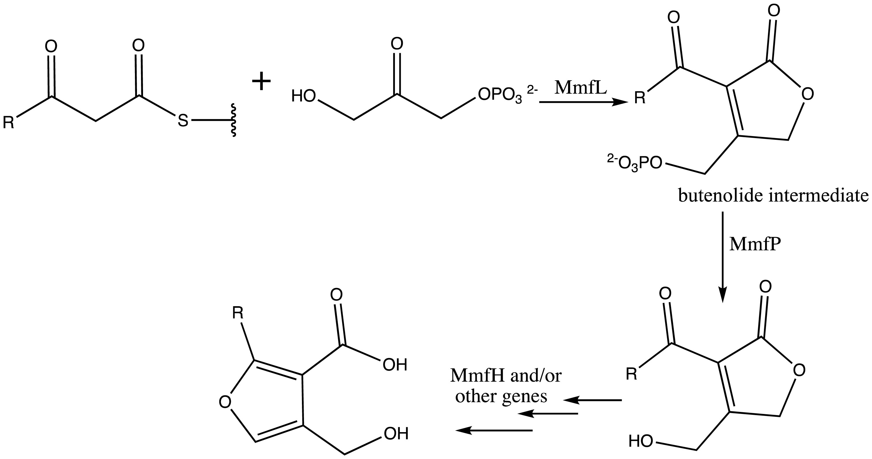
32. Corre C, Song L, O'Rourke S, et al. (2008) 2-Alkyl-4-hydroxymethylfuran-3-carboxylic acids, antibiotic production inducers discovered by Streptomyces coelicolor genome mining. Proc Natl Acad Sci USA 105: 17510–17515.
33. Sidda JD, Corre C (2012) Gamma-butyrolactone and furan signaling systems in Streptomyces. Method Enzymol 517: 71–87.
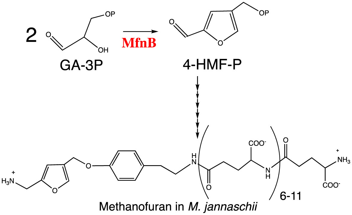
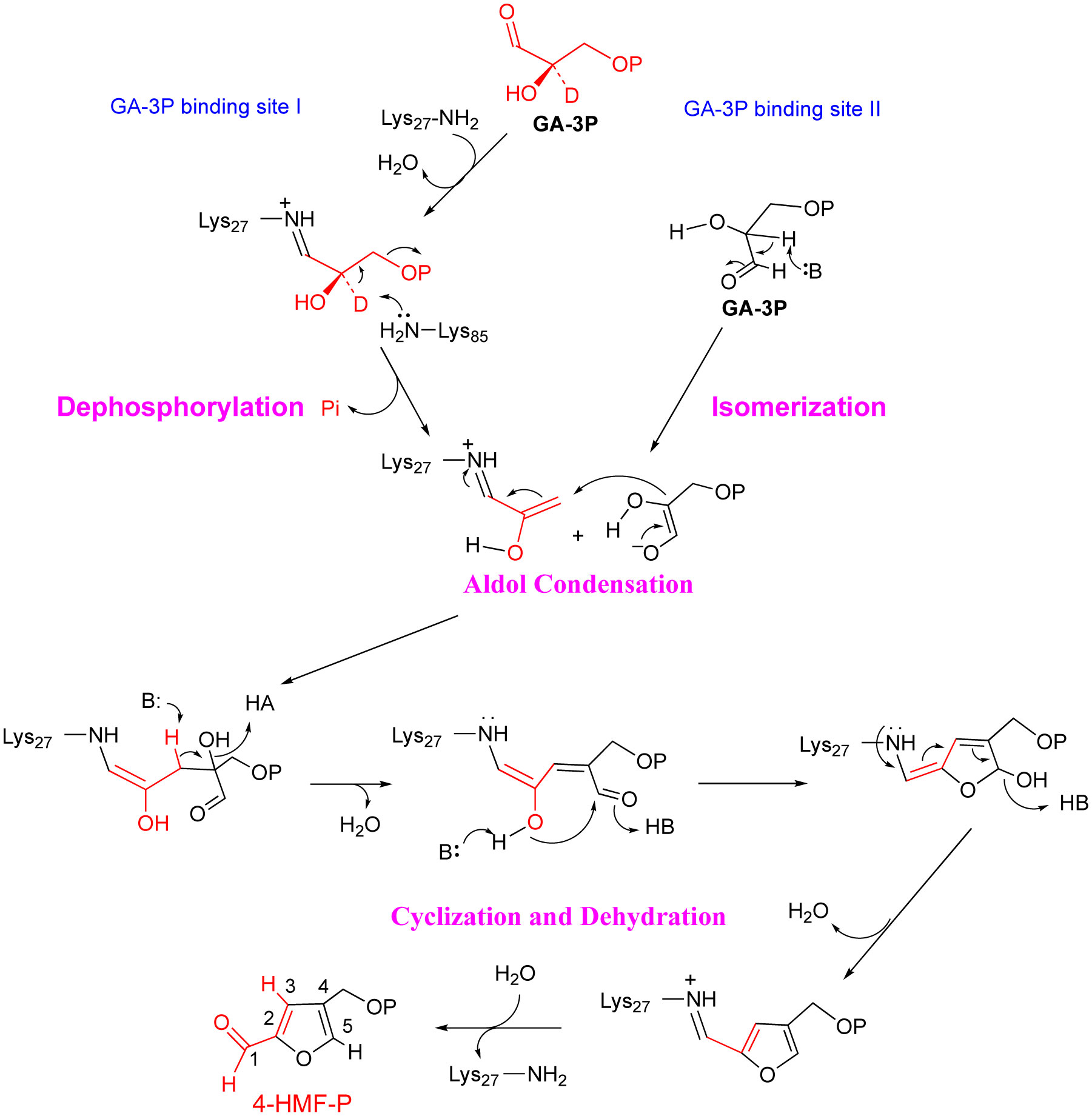
34. Wang Y, Jones MK, Xu H, et al. (2015) Mechanism of the enzymatic synthesis of 4-(Hydroxymethyl)-2-furancarboxaldehyde-phosphate (4-HFC-P) from Glyceraldehyde-3-phosphate catalyzed by 4-HFC-P synthase. Biochemistry 54: 2997–3008.
35. Miller D, Wang Y, Xu H, et al. (2014) Biosynthesis of the 5-(Aminomethyl)-3-furanmethanol moiety of methanofuran. Biochemistry 53: 4635–4647.
36. Wang Y, Xu H, Jones MK, et al. (2015) Identification of the final two genes functioning in methanofuran biosynthesis in Methanocaldococcus jannaschii. J Bacteriol 197: 2850–2858.
37. Jia J, Schorken U, Lindqvist Y, et al. (1997) Crystal structure of the reduced Schiff-base intermediate complex of transaldolase B from Escherichia coli: mechanistic implications for class I aldolases. Protein Sci 6: 119–124.
38. Hester G, Brenner-Holzach O, Rossi FA, et al. (1991) The crystal structure of fructose-1,6-bisphosphate aldolase from Drosophila melanogaster at 2.5 A resolution. FEBS Lett 292: 237–242.
39. Sygusch J, Beaudry D, Allaire M (1987) Molecular architecture of rabbit skeletal muscle aldolase at 2.7-A resolution. Proc Natl Acad Sci USA 84: 7846–7850.
40. Blom N, Sygusch J (1997) Product binding and role of the C-terminal region in class I D-fructose 1,6-bisphosphate aldolase. Nat Struct Biol 4: 36–39.
41. Izard T, Lawrence MC, Malby RL, et al. (1994) The three-dimensional structure of N-acetylneuraminate lyase from Escherichia coli. Structure 2: 361–369.
42. Kim CG, Yu TW, Fryhle CB, et al. (1998) 3-Amino-5-hydroxybenzoic acid synthase, the terminal enzyme in the formation of the precursor of mC7N units in rifamycin and related antibiotics. J Biol Chem 273: 6030–6040.
43. Kim H, Certa U, Dobeli H, et al. (1998) Crystal structure of fructose-1,6-bisphosphate aldolase from the human malaria parasite Plasmodium falciparum. Biochemistry 37: 4388–4396.
44. Bobik TA, Morales EJ, Shin A, et al. (2014) Structure of the methanofuran/methanopterin-biosynthetic enzyme MJ1099 from Methanocaldococcus jannaschii. Acta Crystallogr F 70: 1472–1479.
45. Heine A, DeSantis G, Luz JG, et al. (2001) Observation of covalent intermediates in an enzyme mechanism at atomic resolution. Science 294: 369–374.
46. Almeida JRM, Röder A, Modig T, et al. (2008) NADH- vs NADPH-coupled reduction of 5-hydroxymethyl furfural (HMF) and its implications on product distribution in Saccharomyces cerevisiae. Appl Microbiol Biot 78: 939–945.
47. Palmqvist E, Hahn-Hägerdal B (2000) Fermentation of lignocellulosic hydrolysates. II: inhibitors and mechanisms of inhibition. Bioresource Technol 74: 25–33.
48. Modig T, Lidén G, Taherzadeh MJ (2002) Inhibition effects of furfural on alcohol dehydrogenase, aldehyde dehydrogenase and pyruvate dehydrogenase. Biochem J 363: 769–776.
49. Barciszewski J, Siboska GE, Pedersen BO, et al. (1997) A mechanism for the in vivo formation of N6-furfuryladenine, kinetin, as a secondary oxidative damage product of DNA. FEBS Lett 414: 457–460.
50. Horváth IS, Taherzadeh MJ, Niklasson C, et al. (2001) Effects of furfural on anaerobic continuous cultivation of Saccharomyces cerevisiae. Biotechnol Bioeng 75: 540–549.
51. Palmqvist E, Hahn-Hägerdal B (2000) Fermentation of lignocellulosic hydrolysates. I: inhibition and detoxification. Bioresource Technol 74: 17–24.
52. Nicolaou SA, Gaida SM, Papoutsakis ET (2010) A comparative view of metabolite and substrate stress and tolerance in microbial bioprocessing From biofuels and chemicals, to biocatalysis and bioremediation. Metab Eng 12: 307–331.
53. Wang X, Miller EN, Yomano LP, et al. (2011) Increased furfural tolerance due to overexpression of NADH-dependent oxidoreductase FucO in Escherichia coli strains engineered for the production of ethanol and lactate. Appl Environ Microb 77: 5132–5140.
54. Liu ZL, Blaschek HP (2010) Biomass conversion inhibitors andin situ detoxification, In: Biomass to Biofuels: Strategies for Global Industries, Blackwell Publishing Ltd., 233–259.
55. Liu ZL, Moon J, Andersh BJ, et al. (2008) Multiple gene-mediated NAD(P)H-dependent aldehyde reduction is a mechanism of in situ detoxification of furfural and 5-hydroxymethylfurfural by Saccharomyces cerevisiae. Appl Microbiol Biot 81: 743–753.
56. Nieves LM, Panyon LA, Wang X (2015) Engineering sugar utilization and microbial tolerance toward lignocellulose conversion. Front Bioeng Biotechnol 3: 1–10.
57. Wierckx N, Koopman F, Ruijssenaars HJ, et al. (2011) Microbial degradation of furanic compounds: biochemistry, genetics, and impact. Appl Microbiol Biot 92: 1095–1105.
58. Zhang J, Zhu Z, Wang X, et al. (2010) Biodetoxification of toxins generated from lignocellulose pretreatment using a newly isolated fungus, Amorphotheca resinae ZN1, and the consequent ethanol fermentation. Biotechnol Biofuels 3: 26.
59. Trifonova R, Postma J, Ketelaars JJMH, et al. (2008) Thermally treated grass fibers as colonizable substrate for beneficial bacterial inoculum. Microbial Ecol 56: 561–571.
60. López MJ, Nichols NN, Dien BS, et al. (2004) Isolation of microorganisms for biological detoxification of lignocellulosic hydrolysates. Appl Microbiol Biot 64: 125–131.
61. Boopathy R, Daniels L (1991) Isolation and characterization of a furfural degrading sulfate-reducing bacterium from an anaerobic digester. Curr Microbiol 23: 327–332.
62. Brune G, Schoberth SM, Sahm H (1983) Growth of a strictly anaerobic bacterium on furfural (2-furaldehyde). Appl Environ Microb 46: 1187–1192.
63. Koopman F, Wierckx N, de Winde JH, et al. (2010) Identification and characterization of the furfural and 5-(hydroxymethyl)furfural degradation pathways of Cupriavidus basilensis HMF14. Proc Natl Acad Sci USA 107: 4919–4924.
64. Dijkman WP, Groothuis DE, Fraaije MW (2014) Enzyme-catalyzed oxidation of 5-hydroxymethylfurfural to furan-2,5-dicarboxylic acid. Angew Chem Int Edit 53: 6515–6518.
65. Dijkman WP, Fraaije MW (2014) Discovery and characterization of a 5-Hydroxymethylfurfural oxidase from Methylovorus sp. strain MP688. Appl Environ Microb 80: 1082–1090.
66. Dijkman WP, Binda C, Fraaije MW, et al. (2015) Structure-based enzyme tailoring of 5-hydroxymethylfurfural oxidase. ACS Catal 5: 1833–1839.
67. de Jong E, Dam MA, Sipos L, et al. (2012) Furandicarboxylic acid (fdca), a versatile building block for a very interesting class of polyesters, In: Biobased Monomers, Polymers, and Materials, American Chemical Society, 1–13.

show all references

This article has been cited by:

1. Muhammad Sajid, Xuebing Zhao, Dehua Liu, Production of 2,5-furandicarboxylic acid (FDCA) from 5-hydroxymethylfurfural (HMF): recent progress focusing on the chemical-catalytic routes, Green Chemistry, 2018, 10.1039/C8GC02680G
2. Rachatida Det-udom, Cheunjit Prakitchaiwattana, Thanachan Mahawanich, Autochthonous microbes and their key properties in browning reduction during soy sauce fermentation, LWT, 2019, 10.1016/j.lwt.2019.05.042

Reader Comments

your name: * your email: *

Download full text in PDF

Associated material

Metrics