Citation: Alejandra S. Coronel, Susana R. Feldman, Emliano Jozami, Kehoe Facundo, Rubén D. Piacentini, Marielle Dubbeling, Francisco J. Escobedo. Effects of urban green areas on air temperature in a medium-sized Argentinian city[J]. AIMS Environmental Science, 2015, 2(3): 803-826. doi: 10.3934/environsci.2015.3.803
[1] | Md Nazmul Hassan, Angela Peace . Mechanistically derived Toxicant-mediated predator-prey model under Stoichiometric constraints. Mathematical Biosciences and Engineering, 2020, 17(1): 349-365. doi: 10.3934/mbe.2020019 |
[2] | Jie Hu, Juan Liu, Peter Yuen, Fuzhong Li, Linqiang Deng . Modelling of a seasonally perturbed competitive three species impulsive system. Mathematical Biosciences and Engineering, 2022, 19(3): 3223-3241. doi: 10.3934/mbe.2022149 |
[3] | Ming Chen, Menglin Gong, Jimin Zhang, Lale Asik . Comparison of dynamic behavior between continuous- and discrete-time models of intraguild predation. Mathematical Biosciences and Engineering, 2023, 20(7): 12750-12771. doi: 10.3934/mbe.2023569 |
[4] | Zhenyao Sun, Da Song, Meng Fan . Dynamics of a stoichiometric phytoplankton-zooplankton model with season-driven light intensity. Mathematical Biosciences and Engineering, 2024, 21(8): 6870-6897. doi: 10.3934/mbe.2024301 |
[5] | Lina Hao, Meng Fan, Xin Wang . Effects of nutrient enrichment on coevolution of a stoichiometric producer-grazer system. Mathematical Biosciences and Engineering, 2014, 11(4): 841-875. doi: 10.3934/mbe.2014.11.841 |
[6] | Fang Liu, Yanfei Du . Spatiotemporal dynamics of a diffusive predator-prey model with delay and Allee effect in predator. Mathematical Biosciences and Engineering, 2023, 20(11): 19372-19400. doi: 10.3934/mbe.2023857 |
[7] | Ming Chen, Meng Fan, Congbo Xie, Angela Peace, Hao Wang . Stoichiometric food chain model on discrete time scale. Mathematical Biosciences and Engineering, 2019, 16(1): 101-118. doi: 10.3934/mbe.2019005 |
[8] | Yang Kuang, Jef Huisman, James J. Elser . Stoichiometric Plant-Herbivore Models and Their Interpretation. Mathematical Biosciences and Engineering, 2004, 1(2): 215-222. doi: 10.3934/mbe.2004.1.215 |
[9] | Da Song, Meng Fan, Ming Chen, Hao Wang . Dynamics of a periodic stoichiometric model with application in predicting and controlling algal bloom in Bohai Sea off China. Mathematical Biosciences and Engineering, 2019, 16(1): 119-138. doi: 10.3934/mbe.2019006 |
[10] | Eduardo González-Olivares, Betsabé González-Yañez, Jaime Mena-Lorca, José D. Flores . Uniqueness of limit cycles and multiple attractors in a Gause-typepredator-prey model with nonmonotonic functional response and Allee effecton prey. Mathematical Biosciences and Engineering, 2013, 10(2): 345-367. doi: 10.3934/mbe.2013.10.345 |
Fractional calculus is one of today's most popular mathematical tools to model real-world problems. More specifically, it has been applied to model evolutionary systems involving memory effects on dynamical systems. Partial differential equations (PDEs) with fractional operators are important in describing phenomena in many fields such as physics, biology and chemistry [1,2]. Based on the generalizations of fractional derivatives by famous mathematicians such as Euler, Lagrange, Laplace, Fourier, Abel and Liouville, today's mathematicians have explored and introduced many more types of fractional derivatives such as Riemann-Liouville, Caputo, Liouville, Weyl, Riesz and Hifler [3,4,5,6].
PDEs with conformable derivatives attract interested mathematicians using different approaches because of their wide range of applications, such as electrical circuits[7] and chaotic systems in dynamics[8]. We recognize that the conformable and classical derivatives have a close relationship. There is an interesting observation that: If $ f $ is a real function and $ s > 0 $, then $ f $ has a conformable fractional derivative of order $ \beta $ at $ s $ if and only if it is (classically) differentiable at $ s $, and
$ C∂βf(s)∂sβ=s1−β∂f(s)∂s, $ | (1.1) |
where $ 0 < \beta \leq 1 $. Another surprising observation is that Eq (1.1) will not hold if $ f $ is defined in a general Banach space. We can better understand why the ODEs with the conformable derivative on $ \mathbb{R} $ have been studied so much. In addition, the relevant research in infinite-dimensional spaces, such as Banach or Hilbert space, is still limited, which motivates us to investigate some types of PDEs with conformable derivatives in Hilbert or Sobolev spaces.
Besides, in some phenomena, the conformable derivative is better simulated than the classical derivative. In [9], the authors considered the conformable diffusion equation
$ C∂α∂tαu(x,t)=Dα∂2∂x2u(x,t), $ | (1.2) |
where $ 0 < \alpha \le 1, \, x > 0, \, t > 0, $ $ u(x, t) $ is the concentration, and $ D_\alpha $ represents the generalized diffusion coefficient, which was applied in the description of a subdiffusion process. In particular, the conformable diffusion equation (1.2) reduces to the normal diffusion equation if $ \alpha = 1 $. A natural and fundamental question is, "Does the conformable diffusion model predict better than the normal diffusion model?". The results in [9] show that the conformable derivative model agrees better with the experimental data than the normal diffusion equation.
Let $ \Omega \subset\mathbb{R}^N $ ($ N \ge 1 $) be a bounded domain with smooth boundary $ \partial \Omega $, and $ T > 0 $ is a given positive number. In this paper, we investigate the Sobolev equation with a conformable derivative as follows
$ {C∂α∂tαu+(−Δ)βu(x,t)−mC∂α∂tαΔu=F(u(x,t)),x∈Ω,t∈(0,T),u(x,t)=0,x∈∂Ω,t∈(0,T),u(x,0)=u0(x)x∈Ω $ | (1.3) |
where $ \alpha, \beta \in (0, 1] $, $ m > 0 $, the time fractional derivative $ \frac{{ }^{ C}\partial^\alpha}{\partial t^\alpha} $ is the conformable derivative of order $ \alpha, $ defined in Definition 1. The function $ F $ represents the external forces or the advection term of a diffusion phenomenon, etc., and the function $ u_0 $ is the initial condition specified later. The operator $ (-\Delta)^\beta $ is the fractional Laplacian operator, which is well-defined in [10] (see page 3). In the sense of distribution, the study of weak solutions to Problem (1.3) is still limited compared to the classical problem. Thus, the fundamental knowledge in the distributive sense for Problem (1.3) is still open and challenging, which is the main reason and motivation for us to study the problem from the perspective of the semigroup.
Next, we mention some results related to Problem (1.3). There are two interesting observations regarding Problem (1.3).
$ \bullet $ If we take $ m = 0 $ in Problem (1.3), then we obtain an initial boundary value problem of the parabolic equation with a conformable operator as follows
$ {C∂α∂tαu+(−Δ)βu(x,t)=F(u(x,t)),x∈Ω,t∈(0,T),u(x,t)=0,x∈∂Ω,t∈(0,T),u(x,0)=u0(x)x∈Ω. $ | (1.4) |
The latest results on the well-posedness of solutions to Problem (1.4) are shown in more detail in [11], and the authors used the Hilbert scales space technique to prove the local existence of the mild solution to Problem (1.4).
$ \bullet $ If $ \alpha = 1 $, the main equation of Problem (1.3) becomes the classical equation
$ ut+(−Δ)βu(x,t)−mΔut=F(u(x,t)). $ | (1.5) |
Equation (1.5) is familiar to mathematicians about PDEs, called the pseudo-parabolic equation, also known as the Sobolev equation. The pseudo-parabolic equation describes a series of important physical processes, such as the permeation of a homogeneous liquid through fractured rock, population aggregation and one-way propagation of the nonlinear dispersion length wave [12,13]. Equation (1.5) has been studied extensively; for details, see [12,13,14] and references given there. Concerning the study of the existence and blowup of solutions to pseudo-parabolic equations, we refer the reader to [15,16,17].
For the convenience of readers, we next list some interesting results related to pseudo-parabolic with fractional derivative. Luc et al. in [18] considered fractional pseudo-parabolic equation with Caputo derivative
$ {Dαt(u+kAu)+Aβu=F(t,x,u),in(0,T]×Ω,u(t,x)=0,on(0,T]×∂Ω,u(0,x)=u0(x),inΩ, $ | (1.6) |
where $ 0 < \alpha < 1 $, $ \mathcal A = -\Delta $, $ D^\alpha $ is Caputo fractional derivative operator of order $ \alpha $. They studied the local and global existence of solutions to Problem (1.6) when the nonlinear term $ F $ is the global Lipschitz. Based on the work in [18], there are many related results in the spirit of a semigroup representation of the form of the Fourier series. In [12], the authors studied nonlinear time-fractional pseudo-parabolic equations with Caputo derivative on both bounded and unbounded domains by different methods and techniques from [18]. In [19], the authors studied the nonlocal in time problem for a pseudo-parabolic equation with fractional time and space in the linear case. Tuan et al. [20] derived the nonlinear pseudo-parabolic equation with a nonlocal type of integral condition. In [21], the authors considered the time-space pseudo-parabolic equation with the Riemann-Liouville time-fractional derivative, and they applied the Galerkin method to show the global and local existence of solutions.
As far as we know, there has not been any work that considers the initial boundary value problem (1.3) with a conformable derivative. The main results and methods of the present paper are described in detail as follows
● Firstly, we prove the existence of the global solution to Problem (1.3). The main idea is to use Banach fixed point theorem with the new weighted norm used in [22]. In order to prove the regularity and the derivative of the mild solution, we need to apply some complicated techniques on Hilbert scales for nonlinearity terms.Compared with [11], our method has very different characteristics. It is important to emphasize that proving the existence of the global solution is difficult, which is demonstrated in our current paper, but not in the paper [11].
● Secondly, we investigate the convergence of solution to Problem (1.3) when $ m \to 0^+ $, which does not appear in the works related to fractional pseudo-parabolic equation. This result allows us to get the relationship between the solution of Sobolev equation and parabolic diffusion equation. To overcome the difficulty, we need to control the improper integrals and control the parameters. This pioneering work can open up some new research directions for finding the relationship between the solutions of the pseudo-parabolic equation and the parabolic equation.
● Finally, we prove the convergence of the solution when the order of derivative $ \beta \to 1^- $. This direction of research was motivated by the recent paper [23]. Since the current model has a nonlinear source function, the processing technique for the proof in this paper seems to be more complicated than that of [23].
The greatest difficulty in solving this problem is the study of many integrals containing singular terms, such as $ s^{\alpha-1} $ or $ (t^\alpha- s^\alpha)^{- m} $. To overcome these difficulties, we need to use ingenious calculations and techniques to control the convergence of several generalized integrals.
This paper is organized as follows. Section 2 provides some definitions. In Section 3, we give the definition of the mild solution and some important lemmas for the proof of the main results. Section 4 shows the global existence of the solution to Problem (1.3). In addition, we present the regularity result for the derivative of the mild solution. Section 5 shows the convergence of the solution to Problem (1.3) when $ m \to 0^+ $. In Section 6, we investigate the convergence of mild solutions when $ \beta \to 1^- $.
Definition 2.1. Conformable derivative model: Let $ B $ be a Banach space, and the function $ f:[0, \infty) \to B $. Let $ \frac{{ }^{C}\partial^\beta}{\partial t^\beta} $ be the conformable derivative operator of order $ \beta \in (0, 1] $, locally defined by
$ C∂βf(t)∂tβ:=limh→0f(t+ht1−β)−f(t)hinB $ |
for each $ t > 0 $. (For more details on the above definition, we refer the reader to [24,25,26,27].)
In this section, we introduce the notation and the functional setting used in our paper. Recall the spectral problem
$ {−Δen(x)=λnen(x),x∈Ω,en(x)=0,x∈∂Ω, $ |
admits the eigenvalues $ 0 < \lambda_1 \leq \lambda_2 \leq \dots \leq \lambda_n \leq \dots $ with $ \lambda_n \to \infty $ as $ n \to \infty $. The corresponding eigenfunctions are $ e_n \in H_0^1(\Omega) $.
Definition 2.2. (Hilbert scale space). We recall the Hilbert scale space, which is given as follows
$ Hs(Ω)={f∈L2(Ω)|∞∑n=1λ2sn(∫Ωf(x)en(x)dx)2<∞} $ |
for any $ s \geq 0 $. It is well-known that $ \mathbb H^s (\Omega) $ is a Hilbert space corresponding to the norm
$ \|f\|_{ \mathbb H^s (\Omega)} = \Bigg( \sum\limits_{n = 1}^\infty \lambda_n^{2s} \Big( \int_\Omega f(x) e_n (x){\rm d}x \Big)^2 \Bigg)^{1/2},\; \; f \in \mathbb H^s (\Omega). $ |
Definition 2.3. Let $ {\bf X}_{a, q, \alpha} ((0, T]; B) $ denote the weighted space of all the functions $ \psi \in C ((0, T];X) $ such that
$ ‖ψ‖Xa,q,α((0,T];B):=supt∈(0,T]tae−qtα‖ψ(t,⋅)‖B<∞, $ |
where $ a, q > 0 $ and $ 0 < \alpha \le 1 $ (see [22]). If $ q = 0 $, we denote $ {\bf X}_{a, q} ((0, T]; B) $ by $ {\mathbb X}_{a} ((0, T]; B) $.
In order to find a precise formulation for solutions, we consider the mild solution in terms of the Fourier series
$ u(x,t) = \sum\limits_{n = 1}^\infty \langle u(.,t), e_n \rangle e_n (x). $ |
Taking the inner product of Problem (1.3) with $ e_n $ gives
$ {C∂α∂tα⟨u(.,t),en⟩+λβn⟨u(.,t),en⟩+mλnC∂α∂tα⟨u(.,t),en⟩=⟨F(.,t),en⟩,t∈(0,T),⟨u(.,0),en⟩=⟨u0,en⟩, $ | (3.1) |
where we repeat that
$ \left \langle \Delta u(.,t) , e_n \right \rangle = - \lambda_n \langle u(.,t), e_n \rangle. $ |
The first equation of (3.1) is a differential equation with a conformable derivative as follows
$ C∂α∂tα⟨u(.,t),en⟩+λβn1+mλn⟨u(.,t),en⟩=11+mλn⟨F(.,t),en⟩. $ |
In view of the result in Theorem 5, [26] and Theorem 3.3, [28] the solution to Problem (1.3) is
$ ⟨u(.,t),en⟩=exp(−λβn1+mλntαα)⟨u0,en⟩+11+mλn∫t0να−1exp(λβn1+mλnνα−tαα)⟨F(.,ν),en⟩dν. $ |
To simplify the solution formula, we will express the solution in operator equations. Let us set the following operators
$ Sm,α,β(t)f=∑n∈Nexp(−λβn1+mλntαα)⟨f,en⟩en, $ |
and
$ Pmf=∑n∈N(1+mλn)−1⟨f,en⟩en $ |
for any $ f \in L^2(\Omega) $ in the form $ f = \sum_{n\in \mathbb N} \big\langle f, e_n \big\rangle e_n $. Then the inverse operator of $ {\bf S}_{m, \alpha, \beta}(t) $ is defined by
$ (Sm,α,β(t))−1f=∑n∈Nexp(λβn1+mλntαα)⟨f,en⟩en $ |
The mild solution is given by
$ u(t)=Sm,α,β(t)u0+∫t0να−1PmSm,α,β(t)(Sm,α,β(ν))−1F(ν)dν. $ | (3.2) |
For a qualitative analysis of the solution to (3.2), we need the bounded result for the operators in Hilbert scales space.
Lemma 3.1. (a) Let $ v \in \mathbb H^{s+k-\beta k} (\Omega) $ for any $ k > 0 $. Then we get
$ ‖Sm,α,β(t)v‖Hs(Ω)≤Ckαkm−kt−αk‖v‖Hs+k−βk(Ω), $ | (3.3) |
and for $ 0 \le \nu \le t \le T $,
$ ‖Sm,α,β(t)(Sm,α,β(ν))−1v‖Hs(Ω)≤Ckαkm−k(tα−να)−k‖v‖Hs+k−βk(Ω). $ | (3.4) |
(b) If $ v \in \mathbb H^{s} (\Omega) $, then
$ ‖Sm,α,β(t)v‖Hs(Ω)≤‖v‖Hs(Ω) $ | (3.5) |
and
$ ‖Sm,α,β(t)(Sm,α,β(ν))−1v‖Hs(Ω)≤‖v‖Hs(Ω) $ | (3.6) |
for $ 0 \le \nu \le t \le T $.
(c) If $ v \in \mathbb H^{s} (\Omega) $, then we have
$ \Big\| {\bf P}_m v \Big\|_{\mathbb H^s (\Omega)} \le\big\| v \big\|_{\mathbb H^{s} (\Omega)} $ |
for any $ s $.
Proof. For (a), in view of Parseval's equality, we get that
$ ‖Sm,α,β(t)v‖2Hs(Ω)=∑n∈Nλ2snexp(−2λβn1+mλntαα)⟨v,en⟩2. $ | (3.7) |
Using the inequality $ e^{-y} \le C_k y^{-k} $, we find that
$ exp(−λβn1+mλntαα)≤Ck(λβn1+mλn)−kt−αkα−k=Ckαk(mk+λ−11)λ(1−β)knt−αk, $ | (3.8) |
where we use
$ (1+mλn)k≤Ck(1+mkλkn)≤Ck(mk+λ−11)λkn. $ |
It follows from (3.7) that
$ ‖Sm,α,β(t)v‖2Hs(Ω)≤(Ckαk)2(mk+λ−11)2t−2αk∑n∈Nλ2s+2k−2βkn⟨f,en⟩2=(Ckαk)2(mk+λ−11)2t−2αk‖v‖2Hs+k−βk(Ω). $ |
By a similar explanation, we also get that for $ 0 \le \nu \le t \le T $,
$ ‖Sm,α,β(t)(Sm,α,β(ν))−1v‖2Hs(Ω)=∑n∈Nλ2snexp(λβn1+mλn2να−2tαα)⟨v,en⟩2≤(Ckαk)2(mk+λ−11)2(tα−να)−2k∑n∈Nλ2s+2k−2βkn⟨f,en⟩2=(Ckαk)2(mk+λ−11)2(tα−να)−2k‖v‖2Hs+k−βk(Ω), $ |
where we use the fact that
$ exp(λβn1+mλnνα−tαα)≤Ck(λβn1+mλn)−k(tα−να)−kα−k=Ckαk(mk+λ−11)λ(1−β)kn(tα−να)−k. $ |
Hence, (a) is proved.
For (b), in view of Parseval's equality, we get that
$ ‖Sα,β(t)v‖2Hs(Ω)=∑n∈Nλ2snexp(−2λβn1+mλntαα)⟨v,en⟩2≤∑n∈Nλ2sn⟨v,en⟩2=‖v‖2Hs(Ω), $ |
which allows us to conclude the proof of (3.5). The proof of (3.6) is similar to (3.5), and we omit it here. For (c), noting that $ \left(1+ m \lambda_n \right)^{-1} < 1 $, we can claim it as follows
$ ‖Pmv‖2Hs(Ω)=∑n∈Nλ2sn(1+mλn)−2⟨v,en⟩2≤∑n∈Nλ2sn⟨v,en⟩2=‖v‖2Hs(Ω). $ |
The proof of Lemma 3.1 is completed.
Let $ G: \mathbb H^r (\Omega) \to \mathbb H^s (\Omega) $ such that $ G({\bf 0}) = {\bf 0} $ and
$ ‖G(w1)−G(w2)‖Hs(Ω)≤Lg‖w1−w2‖Hr(Ω), $ | (4.1) |
for any $ w_1, w_2\in \mathbb H^r (\Omega) $ and $ L_g $ is a postive constant.
Theorem 4.1. (i) Let $ G: \mathbb H^r (\Omega) \to \mathbb H^s (\Omega) $ such that (4.1) holds. Here $ r, s $ satisfy that $ s \ge r+k-\beta k $ for $ 0 < k < \frac{1}{2}. $ Let the initial datum $ u_0 \in \mathbb H^{r+k-\beta k} (\Omega) $. Then Problem (1.3) has a unique solution $ u_{m, \alpha, \beta } \in L^p(0, T; \mathbb H^r(\Omega)) $, where
$ 1<p<1b,αk≤b<α−αk. $ |
In addition, we get
$ ‖um,α,β(t)‖Hr(Ω)≤2Ckαk(mk+λ−11)eμ0TαTb−αkt−b‖u0‖Hr+k−βk(Ω), $ | (4.2) |
where $ C_k $ depends on $ k $.
(ii) Let us assume that $ b < \frac{ \alpha}{2} $ and $ u_0 \in \mathbb H^{s+k-\beta k+\beta-1} (\Omega) \cap \mathbb H^{r+k-\beta k} (\Omega) $. Then we have
$ ‖∂∂tum,α,β(.,t)‖Hs(Ω)≲tα−αk−1‖u0‖Hs+k−βk+β−1(Ω)+(tα−1−b+t2α−b−kα−1)‖u0‖Hr+k−βk(Ω). $ | (4.3) |
Here the hidden constant depends on $ k, b, \alpha, m, p, \beta, L_g $ ($ L_g $ is defined in (4.1)).
Proof. Let us define $ { B}: {\bf X}_{b, \mu, \alpha }((0, T]; \mathbb H^r(\Omega)) \to {\bf X}_{b, \mu, \alpha}((0, T]; \mathbb H^r(\Omega)) $, $ \mu > 0 $ by
$ Bw(t):=Sm,α,β(t)u0+∫t0να−1PmSm,α,β(t)(Sm,α,β(ν))−1G(w(ν))dν. $ | (4.4) |
Let the zero function $ w_0(t) = 0 $. From the fact $ G(0) = 0 $, we know that
$ { B} w_0 (t) = {\bf S}_{m, \alpha, \beta}(t) u_0 . $ |
In view of (3.4) as in Lemma 3.3, we obtain the following estimate
$ ‖Bw0(t)‖Hr(Ω))=‖Sm,α,β(t)u0‖Hr(Ω))≤Ckαk(mk+λ−11)t−αk‖u0‖Hr+k−βk(Ω). $ |
Hence, multiplying both sides of the above expression by $ t^b e^{-\mu t^ \alpha} $, we have that
$ tbe−μtα‖Bw0(t)‖Hr(Ω))≤Ckαk(mk+λ−11)tb−αk‖u0‖Hr+k−βk(Ω)≤Ckαk(mk+λ−11)Tb−αk‖u0‖Hr+k−βk(Ω), $ | (4.5) |
where we use $ b \ge \alpha k $. This implies that $ { B} w_0 \in {\bf X}_{b, \mu, \alpha }((0, T]; \mathbb H^r(\Omega)) $. Let any two functions $ w_1, w_2 \in {\bf X}_{b, \mu, \alpha }((0, T]; \mathbb H^r(\Omega)) $. From (4.4) and (3.3), we obtain that
$ ‖Bw1(t)−Bw2(t)‖Hr(Ω))=‖∫t0να−1PmSm,α,β(t)(Sm,α,β(ν))−1(G(w1(ν))−G(w2(ν)))dν‖Hr(Ω))≤Ckαkm−k∫t0να−1(tα−να)−k‖G(w1(ν))−G(w2(ν))‖Hr+k−βk(Ω))dν. $ | (4.6) |
Since the constraint $ s \ge r+k-\beta k $, we know that Sobolev embedding
$ Hs(Ω)↪Hr+k−βk(Ω). $ |
From some above observations and noting (4.1), we get that
$ tbe−μtα‖Bw1(t)−Bw2(t)‖Hr(Ω))≤Ckαk(mk+λ−11)tbe−μtα∫t0να−1(tα−να)−k‖G(w1(ν))−G(w2(ν))‖Hs(Ω))dν≤CkLgαk(mk+λ−11)tbe−μtα∫t0να−1(tα−να)−k‖w1(ν)−w2(ν)‖Hr(Ω))dν=CkLgαk(mk+λ−11)tb∫t0να−1−b(tα−να)−ke−μ(tα−να)νbe−μνα‖w1(ν)−w2(ν)‖Hr(Ω))dν. $ | (4.7) |
From the fact that
$ \Big\| w_1- w_2 \Big\|_{ {\bf X}_{b, \mu, \alpha }((0,T]; \mathbb H^r(\Omega)) } = \sup\limits_{0 \le \nu \le T} \nu^b e^{-\mu \nu^ \alpha } \Big\| w_1(\nu)- w_2(\nu) \Big\|_{\mathbb H^{r}(\Omega)) }, $ |
we follows from (4.7) that
$ sup0≤t≤Ttbe−μtα‖Bw1(t)−Bw2(t)‖Hr(Ω))≤¯C‖w1−w2‖Xb,μ,α((0,T];Hr(Ω))sup0≤t≤T[tb∫t0να−1−b(tα−να)−ke−μ(tα−να)dν], $ | (4.8) |
where $ \overline C = C_k L_g \alpha^k m^{-k}. $ Let us continue to treat the integral term as follows
$ J_{1, \mu} (t) = t^b \int_0^t \nu^{ \alpha-1-b} \left( t^ \alpha-\nu^ \alpha \right)^{-k} e^{-\mu(t^ \alpha-\nu^ \alpha)} {\rm d}\nu. $ |
In order to control the above integral, we need to change the variable $ \nu = t \xi^{\frac{1}{ \alpha}} $. Then we get the following statement
$ J1,μ(t)=1αtα−αk∫10ξ−bα(1−ξ)−ke−μtα(1−ξ)dξ. $ |
Next, we provide the following lemma which can be found in [22], Lemma 8, page 9.
Lemma 4.1. Let $ a_1 > -1 $, $ a_2 > -1 $ such that $ a_1+a_2 \ge -1 $, $ \rho > 0 $ and $ t\in [0, T] $. For $ h > 0 $, the following limit holds
$ limρ→∞(supt∈[0,T]th∫10νa1(1−ν)a2e−ρt(1−ν)dν)=0. $ |
Since $ 0 < b < \alpha $ and $ 0 < k < \min (\frac{b}{ \alpha}, \; \; 1-\frac{b}{ \alpha}) $, we easily to verify that the following conditions hold
$ {α−αk>0,−bα>−1, −k>−1,−bα−k≥−1. $ | (4.9) |
By Lemma 4.1 and (4.9), we have
$ \lim\limits_{\mu \to +\infty } \sup\limits_{0\le t \le T} J_{1, \mu} (t) = 0. $ |
This statement shows that there exists a $ \mu_0 $ such that
$ ¯Csup0≤t≤TJ1,μ0(t)≤12. $ | (4.10) |
Combining (4.8) and (4.10), we obtain
$ ‖Bw1−Bw2‖Xb,μ0((0,T];Hr(Ω))≤12‖w1−w2‖Xb,μ0((0,T];Hr(Ω)) $ | (4.11) |
for any $ w_1, w_2 \in {\bf X}_{b, \mu, \alpha }((0, T]; \mathbb H^r(\Omega)) $. This statement tells us that $ B $ is the mapping from $ {\bf X}_{b, \mu, \alpha }((0, T]; \mathbb H^r(\Omega)) $ to itself. By applying Banach fixed point theorem, we deduce that $ B $ has a fixed point $ u_{m, \alpha, \beta} \in {\bf X}_{b, \mu_0, \alpha}((0, T]; \mathbb H^r(\Omega)) $. Hence, we can see that
$ um,α,β(t)=Sm,α,β(t)u0+∫t0να−1PmSm,α,β(t)(Sm,α,β(ν))−1G(um,α,β(ν))dν. $ | (4.12) |
Let us show the regularity property of the mild solution $ u_{m, \alpha, \beta} $. Indeed, using the triangle inequality and (4.11) and noting that $ B (v = 0) = {\bf S}_{m, \alpha, \beta}(t) u_0 $, we obtain
$ ‖um,α,β‖Xb,μ0,α((0,T];Hr(Ω))=‖Bum,α,β‖Xb,μ0,α((0,T];Hr(Ω))≤12‖um,α,β‖Xb,μ0((0,T];Hr(Ω))+‖B(v=0)‖Xb,μ0,α((0,T];Hr(Ω))=12‖um,α,β‖Xb,μ0,α((0,T];Hr(Ω))+‖Sm,α,β(t)u0‖Xb,μ0,α((0,T];Hr(Ω)), $ |
which combined with (4.5), we get
$ ‖um,α,β‖Xb,μ0,α((0,T];Hr(Ω))≤2Ckαk(mk+λ−11)Tb−αk‖u0‖Hr+k−βk(Ω), $ |
which allows us to get that
$ ‖um,α,β(t)‖Hr(Ω)≤˜C1t−b‖u0‖Hr+k−βk(Ω), $ | (4.13) |
where $ \widetilde C_1 $ depends on $ k, \mu_0, b, \alpha, m $ and
$ \widetilde C_1 = 2 C_k \alpha^k \left(m^k+ \lambda_1^{-1} \right) e^{\mu_0 T^ \alpha} T^{b- \alpha k}, $ |
and we remind that $ C_k $ depends on $ k $. Note that the improper integral $ \int_0^T t^{-pb} {\rm d}t $ is convergent for $ 1 < p < \frac{1}{b} $, we deduce that
$ u_{m, \alpha, \beta} \in L^p(0,T; \mathbb H^r(\Omega) ), $ |
and the following regularity holds
$ ‖um,α,β‖Lp(0,T;Hr(Ω))≤˜C‖u0‖Hr+k−βk(Ω), $ |
where $ \widetilde C $ depends on $ k, \mu_0, b, \alpha, m, p $. Our next aim is to claim the derivative of the mild solution $ u_{m, \alpha, \beta} $. Applying the following formula
$ {\rm d} \left( \int_0^t \mathcal K(t,s) {\rm d}s \right) = \int_0^t \partial_t \mathcal K (t,s) {\rm d}s+ \mathcal K(t,t) {\rm d}t, $ |
we obtain the following equality
$ ∂∂tum,α,β(.,t)=tα−1Qm,α,β(t)u0+tα−1G(um,α,β(x,t))+tα−1∫t0να−1PmQm,α,β(t)(Sm,α,β)−1(ν)G(um,α,β(ν))dν, $ | (4.14) |
where the operator $ {\bf Q}_{m, \alpha, \beta}(t) $ is defined by
$ Qm,α,β(t)v=−∑n∈Nλβn1+mλnexp(−λβn1+mλntαα)⟨v,en⟩en $ |
for any $ v \in L^2(\Omega) $. In view of Parseval's equality, we get that
$ ‖Qm,α,β(t)v‖2Hs(Ω)=∑n∈Nλ2sn(λβn1+mλn)2exp(−2λβn1+mλntαα)⟨v,en⟩2. $ |
Using (3.8) and noting that $ \frac{ \lambda_n^\beta }{1+ m \lambda_n} \le m^{-1} \lambda_n^{\beta-1} $, we get that
$ ‖Qm,α,β(t)v‖2Hs(Ω)≤(Ckαkm−k−1)2t−2αk∑n∈Nλ2s+2k−2βk+2β−2n⟨v,en⟩2, $ |
which implies that
$ ‖Qm,α,β(t)v‖Hs(Ω)≤Ckαkm−k−1t−αk‖v‖Hs+k−βk+β−1(Ω) $ | (4.15) |
for any $ v \in \mathbb H^{s+k-\beta k+\beta-1} (\Omega) $. In a similar technique as above, we also get that
$ ‖Qm,α,β(t)(Sm,α,β)−1(ν)v‖Hs(Ω)≤Ckαkm−k−1(tα−να)−k‖v‖Hs+k−βk+β−1(Ω), $ | (4.16) |
for any $ 0 \le \nu \le t $. Let us go back to the right hand side of (4.14). By (4.15), we evaluate the first term on the right hand side of (4.14) as follows
$ ‖tα−1Qm,α,β(t)u0‖Hs(Ω)≤Ckαkm−k−1tα−αk−1‖u0‖Hs+k−βk+β−1(Ω). $ | (4.17) |
Using global Lipschitz of $ G $ as in (4.1) and the fact that $ G({\bf 0}) = {\bf 0} $, the second term on the right hand side of (4.14) is estimated as follows
$ ‖tα−1G(um,α,β(x,t))‖Hs(Ω)≤˜C1tα−1Lg‖um,α,β‖Hr(Ω)≤˜C1Lgtα−1−b‖u0‖Hr+k−βk(Ω), $ | (4.18) |
where we use (4.13). Let us now to treat the third integral term in (4.14). By (4.16), we obtain that
$ ‖∫t0να−1PmQm,α,β(t)(Sm,α,β)−1(ν)G(um,α,β(ν))dν‖Hs(Ω)≤Ckαkm−k−1∫t0να−1(tα−να)−k‖G(um,α,β(ν))‖Hs+k−βk+β−1(Ω)dν. $ | (4.19) |
Since $ \beta \le 1 $ and $ 0 < k < 1 $, we can easily verify that $ s+k-\beta k+\beta-1 \le s $, which implies the Sobolev embedding $ \mathbb H^{s}(\Omega) \hookrightarrow \mathbb H^{s+k-\beta k+\beta-1 }(\Omega) $ is true. From these above observations and using (4.13), we derive that
$ ∫t0να−1(tα−να)−k‖G(um,α,β(ν))‖Hs+k−βk+β−1(Ω)dν≤C(s,k,β)∫t0να−1(tα−να)−k‖G(um,α,β(ν))‖Hs(Ω)dν≤LgC(s,k,β)∫t0να−1(tα−να)−k‖um,α,β(ν)‖Hr(Ω)dν≤LgC(s,k,β)˜C1‖u0‖Hr+k−βk(Ω)(∫t0να−1−b(tα−να)−kdν). $ | (4.20) |
Let us now treat the integral term on the right hand side of (4.20). Controlling it is really not that simple task. By applying Hölder inequality, we find that
$ (∫t0να−1−b(tα−να)−kdν)2=(∫t0να−12−bνα−12(tα−να)−kdν)2≤(∫t0να−1−2bdν)(∫t0να−1(tα−να)−2kdν)=tα−2bα−2b(∫t0να−1(tα−να)−2kdν), $ | (4.21) |
where $ \alpha > 2b $. By changing to a new variable $ z = \nu^ \alpha $, we derive that $ {\rm d}z = \alpha \nu^{ \alpha-1} {\rm d}\nu $. Hence, we infer that
$ ∫t0να−1(tα−να)−2kdν=1α∫tα0(tα−z)−2kdz=tα(1−2k)α(1−2k), $ | (4.22) |
where we note that $ 0 < k < \frac{1}{2} $. Combining (4.21) and (4.22), we obtain that the following inequality
$ ∫t0να−1−b(tα−να)−kdν≤tα−b−kα√α(1−2k)(α−2b). $ | (4.23) |
By (4.23) and following from (4.19) and (4.20), we have
$ ‖∫t0να−1Qm,α,β(t)(Sm,α,β)−1(ν)G(um,α,β(ν))dν‖Hs(Ω)≤Ckαkm−k−1∫t0να−1(tα−να)−k‖G(um,α,β(ν))‖Hs+k−βk+β−1(Ω)dν≤Ckαkm−k−1LgC(s,k,β)˜C1√α(1−2k)(α−2b)tα−b−kα‖u0‖Hr+k−βk(Ω). $ | (4.24) |
Summarizing the above results (4.14), (4.17), (4.18), (4.24) and using the triangle inequality, we obtain the following assertion
$ ‖∂∂tum,α,β(.,t)‖Hs(Ω)≤‖tα−1Qm,α,β(t)u0‖Hs(Ω)+‖tα−1G(um,α,β(x,t))‖Hs(Ω)+tα−1‖∫t0να−1PmQm,α,β(t)(Sm,α,β)−1(ν)G(um,α,β(ν))dν‖Hs(Ω)≤Ckαkm−k−1tα−αk−1‖u0‖Hs+k−βk+β−1(Ω)+˜C1Lgtα−1−b‖u0‖Hr+k−βk(Ω)+Ckαkm−k−1LgC(s,k,β)˜C1√α(1−2k)(α−2b)t2α−b−kα−1‖u0‖Hr+k−βk(Ω) $ |
which shows (4.3). The proof is completed.
The main purpose of this section is to investigate the convergence of mild solutions to Problem (1.3) when $ m \to 0^+ $. Our result gives us an interesting connection between the solution of the Sobolev equation and the parabolic equation.
Theorem 5.1. Let $ G: \mathbb H^r (\Omega) \to \mathbb H^s (\Omega) $ such that $ G({\bf 0}) = {\bf 0} $ and (4.1) holds. Here $ r, s $ satisfy that $ s \ge r+k-\beta k $ for $ 0 < k < \frac{1}{2}. $ Let the initial datum $ u_0 \in \mathbb H^{r+k-\beta k} (\Omega) $. Let $ u_{m, \alpha, \beta} $ and $ u^*_{ \alpha, \beta} $ be the mild solutions to Problem (1.3) with $ m > 0 $ and $ m = 0 $ respectively. Then we get the following estimate
$ ‖um,α,β(t)−u∗α,β(t)‖Hr(Ω)≲[m2γ−εγ+εl2+mk]T∗(α,γ,l,b,k)E1,α(Lgt), $ |
where $ \alpha k \le b < \frac{ \alpha}{2} $, $ \gamma = \frac{k(1-\beta)+l\left(\beta-\frac{\varepsilon}{2} \right) }{\beta+1-\frac{\varepsilon}{2}} $, $ 0 < l < k (1-\beta) $ and $ 1 < \varepsilon < \min \Big(2, \frac{2k(1-\beta)+2l \beta}{l} \Big) $.
Remark 5.1. Note that $ m^{ \frac{2\gamma- \varepsilon \gamma+\varepsilon l }{2} } + m^{k} $ tends to zero when $ m \to 0^+ $. Hence, we can deduce that $ \Big\| u_{m, \alpha, \beta}(t)- u^*_{ \alpha, \beta}(t) \Big\|_{\mathbb H^{r} (\Omega)} \to 0 $ when $ m \to 0^+ $.
Proof. In the case $ m = 0 $, thanks for the results on [11], the mild solution to Problem (1.3) is given by the following operator equation
$ u∗α,β(t)=S∗α,β(t)u0+∫t0να−1S∗α,β(t)(S∗α,β(ν))−1G(u∗α,β(ν))dν, $ | (5.1) |
where we provide two operators that have the following Fourier series representation as follows
$ S∗α,β(t)f=∑n∈Nexp(−λβntαα)⟨f,en⟩en $ |
and
$ (S∗α,β(ν))−1f=∑n∈Nexp(λβnναα)⟨f,en⟩en. $ |
It's worth emphasizing that the existence of the solution to Equation (5.1) has been demonstrated in [11]. Subtracting (5.1) from (4.12), we get the following equality by some simple calculations
$ um,α,β(t)−u∗α,β(t)=(Sm,α,β(t)−S∗α,β(t))u0+∫t0να−1S∗α,β(t)(S∗α,β(ν))−1(G(um,α,β(ν))−G(u∗α,β(ν)))dν+∫t0να−1[PmSm,α,β(t)(Sm,α,β(ν))−1−PmS∗α,β(t)(S∗α,β(ν))−1]G(um,α,β(ν))dν+∫t0να−1(Pm−I)S∗α,β(t)(S∗α,β(ν))−1G(um,α,β(ν))dν=M1+M2+M3+M4. $ | (5.2) |
Next, we estimate the four terms on the right hand of (5.2) in $ \mathbb H^r(\Omega) $ space. We divide this process into four steps as below.
Step 1. Estimate of $ M_1 $. In view of the inequality $ \Big| e^{-c}- e^{-d} \Big| \le C_\gamma \max (e^{-c}, e^{-d}) |c-d|^\gamma \ \text{with}\ \gamma > 0, $ let $ c = \frac{ \lambda_n^\beta }{1+ m \lambda_n} \frac{ t^ \alpha}{ \alpha} $ and $ d = \lambda_n^\beta \frac{ t^ \alpha}{ \alpha} $, we get the following inequality
$ |exp(−λβn1+mλntαα)−exp(−λβntαα)|≤Cγexp(−λβn1+mλntαα)(λβn−λβn1+mλn)γtαγα−γ≤CγCl(λβn1+mλn)−l(tαα)−l(λβn−λβn1+mλn)γtαγα−γ≤CγClαl−γλ−βln(mλ1+βn)γ(11+mλn)γ−ltαγ−αl $ | (5.3) |
by $ e^{-c} > e^{-d} $ and (3.8).
Here $ \gamma $ and $ l $ are two positive constants that are later chosen. For $ 1 < \varepsilon < 2 $ and any $ z > 0 $, we easily verify that $ (1+z)^{\frac{2}{\varepsilon}} \ge 1+ z > z, $ which implies
$ (1+z)γ−l=(1+z)2εε(γ−l)2>zε(γ−l)2 $ | (5.4) |
for any $ \gamma > l > 0 $.
In (5.4), by choosing $ z = 1+ m \lambda_n $ and after some simple calculation, we have $ \left(1+ m \lambda_n\right)^{\gamma-l} > (m \lambda_n)^{\frac{\varepsilon (\gamma-l)}{2} }, $ which leads to the following inequality
$ (11+mλn)γ−l≤(mλn)ε(l−γ)2. $ | (5.5) |
Combining (5.3) and (5.5), we find that
$ |exp(−λβn1+mλntαα)−exp(−λβntαα)|≤C(α,γ,l)m2γ−εγ+εl2tαγ−αlλ−βl+βγ+γ+ε(l−γ)2n. $ | (5.6) |
Therefore, we have the following estimate
$ ‖(Sm,α,β(t)−S∗α,β(t))u0‖2Hr(Ω))=∑n∈Nλ2rn|exp(−λβn1+mλntαα)−exp(−λβntαα)|2⟨u0,en⟩2≤|C(α,γ,l)|2m2γ−εγ+εlt2αγ−2αl∑n∈Nλ2r−2βl+2βγ+2γ+ε(l−γ)n⟨u0,en⟩2, $ |
which implies that
$ ‖(Sm,α,β(t)−S∗α,β(t))u0‖Hr(Ω))≤C(α,γ,l)m2γ−εγ+εl2tαγ−αl‖u0‖Hr−βl+βγ+γ+ε(l−γ)2(Ω). $ | (5.7) |
Next, we explain how to choose the parameters $ l, \varepsilon, \gamma $. Since $ \beta < 1 $, we can choose $ l $ such that
$ 0<l<min(k(1−β),1−ββk)=k(1−β), $ |
which implies that $ 2k(1-\beta)+2l \beta > l $, that is $ \frac{2k(1-\beta)+2l \beta}{l} > 1 $. Then we can choose $ \varepsilon $ such that
$ 1<ε<min(2,2k(1−β)+2lβl). $ |
Let us choose $ \gamma $ such that
$ γ=k(1−β)+l(β−ε2)β+1−ε2. $ |
It is easy to verify that $ \gamma > \frac{l+l\left(\beta-\frac{\varepsilon}{2} \right) }{\beta+1-\frac{\varepsilon}{2}} = l $ and the following equality
$ r-\beta l + \beta \gamma+ \gamma + \frac{\varepsilon (l-\gamma)}{2} = r+k-\beta k. $ |
Then the estimate (5.7) becomes
$ ‖M1‖Hr(Ω)=‖(Sm,α,β(t)−S∗α,β(t))u0‖Hr(Ω))≤C(α,γ,l)m2γ−εγ+εl2tαγ−αl‖u0‖Hr+k−βk(Ω). $ | (5.8) |
Step 2. Estimate of $ M_2 $. Let $ \psi \in \mathbb H^r (\Omega) $. For $ 0 \le \nu \le t \le T $, we can also get
$ ‖S∗α,β(t)(S∗α,β(ν))−1ψ‖2Hr(Ω)=∑n∈Nλ2rnexp(2λβnνα−tαα)⟨ψ,en⟩2≤‖ψ‖2Hr(Ω), $ | (5.9) |
where we use that
$ exp(λβn1+mλnνα−tαα)≤1. $ |
By (5.9) and Sobolev embedding $ \mathbb H^{s}(\Omega)) \hookrightarrow \mathbb H^{r}(\Omega) $, we find that
$ ‖∫t0να−1S∗α,β(t)(S∗α,β(ν))−1(G(um,α,β(ν))−G(u∗α,β(ν)))dν‖Hr(Ω)≤∫t0να−1‖G(um,α,β(ν))−G(u∗α,β(ν))‖Hr(Ω)dν≤C(r,s)∫t0να−1‖G(um,α,β(ν))−G(u∗α,β(ν))‖Hs(Ω)dν. $ | (5.10) |
By the global Lipschitz property of $ G $ as in (4.1) and noting (5.10), it follows that
$ ‖M2‖Hr(Ω)≤LgC(r,s)∫t0να−1‖um,α,β(ν)−u∗α,β(ν)‖Hr(Ω)dν. $ | (5.11) |
Step 3. Estimate of $ M_3 $. Let $ f \in \mathbb H^{r+k-\beta k } (\Omega) $. Then using Parseval' s equality, we have the following identity
$ ‖[PmSm,α,β(t)(Sm,α,β(ν))−1−PmS∗α,β(t)(S∗α,β(ν))−1]f‖2Hr(Ω))=∑n∈Nλ2rn(1+mλn)2|exp(−λβn1+mλntα−ναα)−exp(−λβntα−ναα)|2⟨f,en⟩2. $ | (5.12) |
By a similar explanation as in (5.6), we find that
$ |exp(−λβn1+mλntα−ναα)−exp(−λβntα−ναα)|≤C(α,γ,l)m2γ−εγ+εl2(tα−να)γ−lλ−βl+βγ+γ+ε(l−γ)2n. $ | (5.13) |
By (5.12) and (5.13), we get that
$ ‖[PmSm,α,β(t)(Sm,α,β(ν))−1−PmS∗α,β(t)(S∗α,β(ν))−1]f‖Hr(Ω))≤C(α,γ,l)m2γ−εγ+εl2(tα−να)γ−l‖f‖Hr+k−βk(Ω). $ | (5.14) |
In view of (5.14) and $ s \ge r+k -\beta k $, we derive that
$ ‖[PmSm,α,β(t)(Sm,α,β(ν))−1−PmS∗α,β(t)(S∗α,β(ν))−1]G(u∗α,β(ν))‖Hr(Ω))≤C(α,γ,l)m2γ−εγ+εl2(tα−να)γ−l‖G(um,α,β(ν))‖Hr+k−βk(Ω)≤C(α,γ,l,s)m2γ−εγ+εl2(tα−να)γ−l‖G(um,α,β(ν))‖Hs(Ω). $ | (5.15) |
By using global Lipschitz property of $ G $ as in (4.1) and noting (4.2), we infer that
$ ‖G(um,α,β(ν))‖Hs(Ω)≤Lg‖um,α,β(ν)‖Hr(Ω)≤2CkLgαk(mk+λ−11)eμ0TαTb−αkν−b‖u0‖Hr+k−βk(Ω)≲(mk+λ−11)ν−b‖u0‖Hr+k−βk(Ω), $ | (5.16) |
where the hidden constant depends on $ k, \alpha, L_g, \mu_0, b $. Combining (5.15) and (5.16), we get the following estimate
$ ‖M3‖Hr(Ω)≲m2γ−εγ+εl2(mk+λ−11)‖u0‖Hr+k−βk(Ω)∫t0να−1−b(tα−να)γ−ldν. $ | (5.17) |
Since $ \gamma > l $ and noting that $ b < \alpha $, we infer that
$ ∫t0να−1−b(tα−να)γ−ldν≤tα(γ−l)∫t0να−1−bdν=tα(γ−l)+α−bα−b. $ | (5.18) |
By (5.17) and (5.18), we obtain
$ ‖M3‖Hr(Ω)≲m2γ−εγ+εl2(mk+λ−11)tα(γ−l)+α−bα−b‖u0‖Hr+k−βk(Ω). $ | (5.19) |
Step 4. Estimate of $ M_4 $. By Parseval's equality, we know that
$ ‖(Pm−I)S∗α,β(t)(S∗α,β(ν))−1f‖2Hr(Ω))=∑n∈Nλ2rn(mλn1+mλn)2exp(−2λβntα−ναα)⟨f,en⟩2. $ | (5.20) |
Using the inequality $ e^{-z} \le C(\varepsilon_0) z^{-\varepsilon_0} $, we get the following inequality
$ exp(−2λβntα−ναα)≤C(ε0,α)λ−2βε0n(tα−να)−2ε0. $ | (5.21) |
By the inequality $ (1+z)^2 > z^{\varepsilon_1} $ for $ 1 < \varepsilon_1 < 2 $, we find that the following inequality
$ (mλn1+mλn)2≤m2−ε1λ2−ε1n. $ | (5.22) |
By (5.20)–(5.22), we derive that
$ ‖(Pm−I)S∗α,β(t)(S∗α,β(ν))−1f‖2Hr(Ω))≤C(ε0,α)m2−ε1(tα−να)−2ε0∑n∈Nλ2r+2−ε1−2βε0n⟨f,en⟩2. $ |
Hence, by using Parseval's equality, we obtain the following estimate
$ ‖(Pm−I)S∗α,β(t)(S∗α,β(ν))−1f‖Hr(Ω))≤C(ε0,α)m1−ε12(tα−να)−ε0‖f‖Hr−βε0+1−ε12(Ω)). $ | (5.23) |
Next, we need to choose the appropriate parameters $ \varepsilon_0, \varepsilon_1 $. Let $ \varepsilon_0 = k \in (0, \frac{1}{2}) $ and $ \varepsilon_1 = 2-2k $, we can verify that $ 1 < \varepsilon_1 < 2 $. Hence, it follows from (5.23) that
$ ‖(Pm−I)S∗α,β(t)(S∗α,β(ν))−1f‖Hr(Ω))≤C(k,α)mk(tα−να)−k‖f‖Hr−βk+k(Ω)). $ |
By (5.16) and Sobolev embedding $ \mathbb H^{s}(\Omega)) \hookrightarrow \mathbb H^{r-\beta k +k}(\Omega), $ we derive that
$ ‖(Pm−I)S∗α,β(t)(S∗α,β(ν))−1G(um,α,β(ν))‖Hr(Ω))≤C(k,α)mk(tα−να)−k‖G(um,α,β(ν))‖Hr−βk+k(Ω))≤C(k,α,s)mk(tα−να)−k‖G(um,α,β(ν))‖Hs(Ω))≲mk(tα−να)−k(mk+λ−11)ν−b‖u0‖Hr+k−βk(Ω), $ |
which implies that
$ ‖M4‖Hr(Ω)≲mk(mk+λ−11)‖u0‖Hr+k−βk(Ω)∫t0να−1−b(tα−να)−kdν≲mk(mk+λ−11)tα−b−kα√α(1−2k)(α−2b)‖u0‖Hr+k−βk(Ω), $ | (5.24) |
where we use (4.23). Combining (5.8), (5.11), (5.19) and (5.24), we obtain that
$ ‖um,α,β(t)−u∗α,β(t)‖Hr(Ω)≲‖M1‖Hr(Ω)+‖M2‖Hr(Ω)+‖M3‖Hr(Ω)+‖M4‖Hr(Ω)≤C(α,γ,l)m2γ−εγ+εl2tαγ−αl‖u0‖Hr+k−βk(Ω)+m2γ−εγ+εl2(mk+λ−11)tα(γ−l)+α−bα−b‖u0‖Hr+k−βk(Ω)+mk(mk+λ−11)tα−b−kα√α(1−2k)(α−2b)‖u0‖Hr+k−βk(Ω)+LgC(r,s)∫t0να−1‖um,α,β(ν)−u∗α,β(ν)‖Hr(Ω)dν. $ | (5.25) |
Here we note that $ 1-2k > 0 $ and $ \alpha-2b > 0 $. Since the fact that $ \gamma > l $ and $ b < \min (\alpha, (1-k) \alpha) $, it is obvious to see that
$ t^{ \alpha \gamma- \alpha l} \le T^{ \alpha \gamma- \alpha l}, $ |
$ \frac{t^{ \alpha(\gamma-l)+ \alpha-b}}{ \alpha-b} \le \frac{T^{ \alpha(\gamma-l)+ \alpha-b}}{ \alpha-b}, $ |
$ \frac{t^{ \alpha-b-k \alpha}}{ \sqrt{ \alpha (1-2k) ( \alpha-2b)} } \le \frac{T^{ \alpha-b-k \alpha}}{ \sqrt{ \alpha (1-2k) ( \alpha-2b)} }, $ |
which motivate us to put
$ \mathbb T^*( \alpha, \gamma, l, b, k) = \max \Big( T^{ \alpha \gamma- \alpha l},\; \frac{T^{ \alpha(\gamma-l)+ \alpha-b}}{ \alpha-b}, \frac{T^{ \alpha-b-k \alpha}}{ \sqrt{ \alpha (1-2k) ( \alpha-2b)} } \Big) . $ |
It follows from (5.25) that
$ ‖um,α,β(t)−u∗α,β(t)‖Hr(Ω)≲[m2γ−εγ+εl2+mk]T∗(α,γ,l,b,k)+Lg∫t0να−1‖um,α,β(ν)−u∗α,β(ν)‖Hr(Ω)dν. $ | (5.26) |
To continue to go further in the proof, we now need to recall the following Lemma introduced in [29].
Lemma 5.1. Let $ v \in L^1[0, T] $. Consider some postive constant $ A, B, \beta', \gamma' $ such that $ \beta'+\gamma' > 1 $ and
$ v(t)≤A+B∫t0(t−r)β′−1rγ′−1v(r)dr. $ |
Then for $ 0 < t \le T $, we get
$ v(t)≤AEβ′,γ′(B(Γ(β′))1β′+γ′−1t) $ |
Looking Lemma 5.1 and (5.26), we set
$ v(t) = \Big\| u_{m, \alpha, \beta}(t)- u^*_{ \alpha, \beta}(t) \Big\|_{\mathbb H^{r} (\Omega)},\; \; A = \Big[ m^{ \frac{2\gamma- \varepsilon \gamma+\varepsilon l }{2} } + m^{ \frac{2\gamma- \varepsilon \gamma+\varepsilon l }{2} } + m^{k} \Big] \mathbb T^*( \alpha, \gamma, l, b, k), $ |
$ B = L_g, \; \; \beta' = 1 $ and $ \gamma' = \alpha. $ Then we deduce that
$ ‖um,α,β(t)−u∗α,β(t)‖Hr(Ω)≲[m2γ−εγ+εl2+mk]T∗(α,γ,l,b,k)E1,α(Lgt). $ |
The proof of Theorem 5.1 is completed.
Theorem 6.1. Let $ G: \mathbb H^r (\Omega) \to \mathbb H^s (\Omega) $ such that (4.1) holds. Here $ r, s $ satisfy that $ s > r+k-\beta k $ for $ 0 < k < \frac{1}{2}. $ Let the initial datum $ u_0 \in \mathbb H^{r+k-\beta k+ \varepsilon} (\Omega) $ for any $ \varepsilon > 0 $. Then we get the following estimate
$ ‖um,α,β−u∗∗m,α‖Xαk(0,T;Hr(Ω))≲Dβ(ε,k)‖u0‖Hr+k−βk+ε(Ω)+|Eβ(r,s,k)|‖u0‖Hr+k−βk(Ω), $ |
where the hidden constants depends on $ \alpha, k, T, b $. Here
$ {\bf D}_\beta (\varepsilon,k) = \left| 1- \lambda_1^{1-\beta} \right|^{\frac{ 2k-\beta k+ \varepsilon}{\beta}} + (1-\beta)^{ \varepsilon } , \quad \quad {\bf E}_\beta (r,s,k) = \left| 1- \lambda_1^{1-\beta} \right|^{\frac{ k+s-r}{\beta}} + (1-\beta)^{ s- r-k +\beta k} $ |
for any $ \varepsilon > 0 $.
Proof. For $ m > 0 $, let $ u_{m, \alpha, \beta} $ and $ u^{**}_{m, \alpha} $ be the mild solutions to Problem (1.3) with $ 0 < \beta < 1 $ and $ \beta = 1 $ respectively. Let us recall the formula of these two solutions
$ um,α,β(t):=Sm,α,β(t)u0+∫t0να−1PmSm,α,β(t)(Sm,α,β(ν))−1G(um,α,β(ν))dν. $ | (6.1) |
and
$ u∗∗m,α(t):=Sm,α,1(t)u0+∫t0να−1PmSm,α,1(t)(Sm,α,1(ν))−1G(u∗∗m,α(ν))dν. $ | (6.2) |
Subtracting (6.1) from (6.2) on each side, we derive that
$ um,α,β(t)−u∗∗m,α(t)=(Sm,α,β(t)u0−Sm,α,1(t)u0)+∫t0να−1[PmSm,α,β(t)(Sm,α,β(ν))−1−PmSm,α,1(t)(Sm,α,1(ν))−1]G(u∗∗m,α(ν))dν+∫t0να−1PmSm,α,β(t)(Sm,α,β(ν))−1[G(um,α,β(ν))−G(u∗∗m,α(ν))]dν=N1+N2+N3. $ | (6.3) |
Step 1. Estimate of $ N_1 $. By Parseval' s equality, we have that the following equality
$ ‖N1‖2Hr(Ω)=‖(Sm,α,β(t)u0−Sm,α,1(t)u0)‖2Hr(Ω)=∑n∈Nλ2rn|exp(−λβn1+mλntαα)−exp(−λn1+mλntαα)|2⟨u0,en⟩2=∑λn>1λ2rn|exp(−λβn1+mλntαα)−exp(−λn1+mλntαα)|2⟨u0,en⟩2+∑λn≤1λ2rn|exp(−λβn1+mλntαα)−exp(−λn1+mλntαα)|2⟨u0,en⟩2=N1,1+N1,2. $ | (6.4) |
For the term $ N_{1, 1} $, since $ \lambda_n > 1 $ and $ 0 < \beta < 1 $, we note that $ \frac{ \lambda_n^\beta }{1+ m \lambda_n} < \frac{ \lambda_n }{1+ m \lambda_n} $. Hence, we have the following inequality
$ \exp\left( - \frac{ \lambda_n^\beta }{1+ m \lambda_n} \frac{ t^ \alpha}{ \alpha} \right) > \exp\left( - \frac{ \lambda_n }{1+ m \lambda_n} \frac{ t^ \alpha}{ \alpha} \right) . $ |
In view of the above inequality
$ \Big| e^{-c}- e^{-d} \Big| \le C_{\gamma'} \max (e^{-c}, e^{-d}) |c-d|^{\gamma'},\; \; \; \gamma' > 0 $ |
with $ c = \exp\left(- \frac{ \lambda_n^\beta }{1+ m \lambda_n} \frac{ t^ \alpha}{ \alpha} \right) $ and $ d = \exp\left(- \frac{ \lambda_n }{1+ m \lambda_n} \frac{ t^ \alpha}{ \alpha} \right) $, we derive that
$ |exp(−λβn1+mλntαα)−exp(−λn1+mλntαα)|≤Cγ′exp(−λβn1+mλntαα)|λn−λβn1+mλn|γ′≤C(γ′,ε′)(λβn1+mλntαα)−ε′|λn−λβn1+mλn|γ′=C(γ′,ε′)α−ε′t−αε′(1+mλn)ε′−γ′λ−βε′n|λn−λβn|γ′. $ | (6.5) |
Since the fact that $ \lambda_n > 1 $, we know that $ \Big| \lambda_n- \lambda_n^\beta \Big|^{\gamma'} = \lambda_n^{ \gamma'} \left(1- \lambda_n^{\beta-1} \right)^{\gamma'}. $ Using the inequality $ 1- e^{-y} \le C(\mu) y^\mu $ for any $ \mu > 0 $, we find that
$ 1−λβ−1n=1−exp[−(1−β)log(λn)]≤C(μ)(1−β)μlogμ(λn)≤C(μ)(1−β)μλμn, $ |
where we note that $ 0 < \log(y) \le y $ for any $ y > 1 $, which implies that
$ |λn−λβn|γ′=λγ′n(1−λβ−1n)γ′≤C(μ,γ′)(1−β)μγ′λμγ′+γ′n. $ | (6.6) |
Combining (6.5) and (6.6), we derive that
$ |exp(−λβn1+mλntαα)−exp(−λn1+mλntαα)|≤C(μ,γ′,ε′)α−ε′t−αε′(1+mλn)ε′−γ′(1−β)μγ′λ−βε′nλμγ′+γ′n. $ |
If we make the assumption $ \varepsilon' \le \gamma' $, then $ \left(1+ m \lambda_n \right)^{\varepsilon'-\gamma'} \le 1 $, which allows us to obtain that
$ N1,1≤|C(μ,γ′,ε′,α)|2t−2αε′(1−β)2μγ′∑λn>1λ2r+2μγ′+2γ′−2βε′n⟨u0,en⟩2≤|C(μ,γ′,ε′,α)|2t−2αε′(1−β)2μγ′‖u0‖2Hr+μγ′+γ′−βε′(Ω). $ |
Let us choose $ \mu = \frac{\varepsilon}{k} $ and $ \gamma' = \varepsilon' = k $ for any $ \varepsilon > 0 $. Then we get the following estimate
$ N1,1≤|C(ε,k,α)|2t−2αk(1−β)2ε‖u0‖2Hr+k−βk+ε(Ω). $ | (6.7) |
Before mention to $ N_{1, 2} $, we provide a set $ \overline N = \Big\{ n \in \mathbb N: \lambda_n \le 1 \Big\}. $ Let us give the observation that if $ \overline N $ is an empty set, then $ N_{1, 2} = 0 $. If $ \overline N $ is a non-empty set, then $ \lambda_1 \le 1 $. For the term $ N_{1, 2} $, we note that $ \frac{ \lambda_n^\beta }{1+ m \lambda_n} > \frac{ \lambda_n }{1+ m \lambda_n} $ since $ \lambda_n \le 1 $ and $ 0 < \beta < 1 $. Hence, we have that
$ \exp\left( - \frac{ \lambda_n^\beta }{1+ m \lambda_n} \frac{ t^ \alpha}{ \alpha} \right) < \exp\left( - \frac{ \lambda_n }{1+ m \lambda_n} \frac{ t^ \alpha}{ \alpha} \right) . $ |
By using the fact that
$ \Big| e^{-c}- e^{-d} \Big| \le C_{\gamma_1} \max (e^{-c}, e^{-d}) |c-d|^{\gamma_1},\; \; \; \gamma_1 > 0 $ |
with $ c = \exp\left(- \frac{ \lambda_n^\beta }{1+ m \lambda_n} \frac{ t^ \alpha}{ \alpha} \right) $ and $ d = \exp\left(- \frac{ \lambda_n }{1+ m \lambda_n} \frac{ t^ \alpha}{ \alpha} \right) $, we derive that
$ |exp(−λβn1+mλntαα)−exp(−λn1+mλntαα)|≤C(γ1)exp(−λn1+mλntαα)|λn−λβn1+mλn|γ1≤C(γ1,ε1)(λn1+mλntαα)−ε1|λn−λβn1+mλn|γ1=C(γ1,ε1)α−ε1t−αε1(1+mλn)ε1−γ1λ−ε1n|λn−λβn|γ1. $ | (6.8) |
Since $ \lambda_1 \le \lambda_n \le 1 $, it is obvious to see that
$ |λn−λβn|γ1=(λβn−λn)γ1=λβγ1n|1−λ1−βn|γ1≤λβγ1n|1−λ1−β1|γ1. $ | (6.9) |
Combining (6.8) and (6.9), we find that
$ |exp(−λβn1+mλntαα)−exp(−λn1+mλntαα)|≤C(γ1,ε1,α)|1−λ1−β1|γ1t−αε1(1+mλn)ε1−γ1λ−ε1+βγ1n. $ | (6.10) |
Hence, it follows from (6.10) that
$ N1,2=∑λn≤1λ2rn|exp(−λβn1+mλntαα)−exp(−λn1+mλntαα)|2⟨u0,en⟩2≤|C(γ1,ε1,α)|2|1−λ1−β1|2γ1t−2αε1∞∑n=1(1+mλn)2ε1−2γ1λ2r−2ε1+2βγ1n⟨u0,en⟩2. $ |
Let $ \varepsilon_1 = k $ and $ \gamma_1 = \frac{2k+\varepsilon }{\beta}-k $. Since $ 0 < \beta < 1 $, we know that
$ \varepsilon_1 < \gamma_1 , \quad 2r-2\varepsilon_1+ 2\beta \gamma_1 = 2r+2k-2\beta k +2\varepsilon. $ |
Hence, in view of Parseval's equality, we get the following estimate
$ N1,2≤C(k,r,ε,α)|1−λ1−β1|4k−2βk+2εβt−2αk‖u0‖2Hr+k−βk+ε(Ω). $ | (6.11) |
Combining (6.4), (6.7) and (6.11), we obtain the following estimate
$ ‖N1‖2Hr(Ω)=N1,1+N1,2≤C(k,r,ε,α)[|1−λ1−β1|4k−2βk+2εβ+(1−β)2ε]t−2αk‖u0‖2Hr+k−βk+ε(Ω). $ |
By taking the square root of both sides of the above expression and using the inequality $ \sqrt{a+b} \le \sqrt{a}+ \sqrt{b} $ for any $ a, b \ge 0 $, we get
$ ‖N1‖Hr(Ω)≤C(k,r,ε,α)Dβ(ε,k)t−αk‖u0‖Hr+k−βk+ε(Ω). $ | (6.12) |
Here we denote
$ {\bf D}_\beta (\varepsilon,k) = \left| 1- \lambda_1^{1-\beta} \right|^{\frac{ 2k-\beta k+ \varepsilon}{\beta}} + (1-\beta)^{ \varepsilon } , \quad \varepsilon > 0, $ |
where we observe that $ {\bf D}_\beta (\varepsilon, k) \to 0, \ \beta \to 1^{-}. $
Step 2. Estimate of $ N_2 $. We confirm the following result for any $ \varepsilon_0 > 0 $ using the method similar to Step 1,
$ ‖[PmSm,α,β(t)(Sm,α,β(ν))−1−PmSm,α,1(t)(Sm,α,1(ν))−1]ψ‖Hr(Ω)≤C(k,r,ε0,α)[|1−λ1−β1|2k−βk+ε0β+(1−β)ε0](tα−να)−k‖ψ‖Hr+k−βk+ε0(Ω). $ |
Since $ s > r+k-\beta k $, we know that $ \varepsilon_0 = s- r-k +\beta k > 0 $, and using global Lipschitz property of $ G $, we derive that
$ ‖[PmSm,α,β(t)(Sm,α,β(ν))−1−PmSm,α,1(t)(Sm,α,1(ν))−1]G(u∗∗m,α(ν))‖Hr(Ω)≤¯C1Eβ(r,s,k)(tα−να)−k‖G(u∗∗m,α(ν))‖Hs(Ω)≤Kg¯C1Eβ(r,s,k)(tα−να)−k‖u∗∗m,α(ν)‖Hr(Ω), $ |
where $ \overline C_1 = C (k, r, s, \beta, \alpha) $, and we have the following observation
$ \quad {\bf E}_\beta (r,s,k) = \left| 1- \lambda_1^{1-\beta} \right|^{\frac{ k+s-r}{\beta}} + (1-\beta)^{ s- r-k +\beta k} \to 0, \quad \beta \to 1^{-}. $ |
In view of (4.2), we obtain that the following upper bound
$ ‖u∗∗m,α(ν)‖Hr(Ω)≤¯C2ν−b‖u0‖Hr+k−βk(Ω), $ |
where $ \overline C_2 = C(k, \alpha, m, \mu_0, T, b). $ From two latter estimations as above, we infer that
$ ‖N2‖Hr(Ω)≤∫t0να−1‖[PmSm,α,β(t)(Sm,α,β(ν))−1−PmSm,α,1(t)(Sm,α,1(ν))−1]G(u∗∗m,α(ν))‖Hr(Ω)dν≤¯C3Eβ(r,s,k)‖u0‖Hr+k−βk(Ω)∫t0να−1−b(tα−να)−kdν, $ | (6.13) |
where $ \overline C_3 = K_g \overline C_1 \overline C_2 $. Using (4.23), we obtain that the following inequality
$ ∫t0να−1−b(tα−να)−kdν≤tα−b−kα√α(1−2k)(α−2b). $ | (6.14) |
Combining (6.13) and (6.14), we obtain that
$ ‖N2‖Hr(Ω)≤¯C3tα−b−kα√α(1−2k)(α−2b)Eβ(r,s,k)‖u0‖Hr+k−βk(Ω). $ | (6.15) |
Step 3. Estimate of $ N_3 $. By a similar argument as in (4.6), we find that
$ ‖∫t0να−1PmSm,α,β(t)(Sm,α,β(ν))−1[G(um,α,β(ν))−G(u∗∗m,α(ν))]dν‖Hr(Ω))≤Ckαkm−k∫t0να−1(tα−να)−k‖G(um,α,β(ν))−G(u∗∗m,α(ν))‖Hr+k−βk(Ω))dν. $ |
Since $ s > r+k-\beta k $ and using global Lipschitz property of $ G $, we obtain that
$ ‖G(um,α,β(ν))−G(u∗∗m,α(ν))‖Hr+k−βk(Ω))≤‖G(um,α,β(ν))−G(u∗∗m,α(ν))‖Hs(Ω))≤Kg‖um,α,β(ν)−u∗∗m,α(ν)‖Hr(Ω)). $ |
From the two above observations, we confirm the following statement
$ ‖N3‖Hr(Ω)≤¯C3∫t0να−1(tα−να)−k‖um,α,β(ν)−u∗∗m,α(ν)‖Hr(Ω))dν, $ | (6.16) |
where $ \overline C_3 = C_k \alpha^k m^{-k}K_g. $ Combining (6.3), (6.12), (6.15) and (6.16), we deduce the following estimate
$ ‖um,α,β(t)−u∗∗m,α(t)‖Hr(Ω)≤‖N1‖Hr(Ω)+‖N2‖Hr(Ω)+‖N3‖Hr(Ω)≤˜Ct−αkDβ(ε,k)‖u0‖Hr+k−βk+ε(Ω)+¯C3tα−b−kα√α(1−2k)(α−2b)Eβ(r,s,k)‖u0‖Hr+k−βk(Ω)+¯C3∫t0να−1(tα−να)−k‖um,α,β(ν)−u∗∗m,α(ν)‖Hr(Ω))dν, $ | (6.17) |
where $ \widetilde C = C (k, r, \varepsilon, \alpha) $. By the Hölder inequality and in combination with (4.22), we get the estimate of the third term on the right hand side of (6.17) as follows
$ (∫t0να−1(tα−να)−k‖um,α,β(ν)−u∗∗m,α(ν)‖Hr(Ω))dν)2≤(∫t0να−1(tα−να)−2kdν)(∫t0να−1‖um,α,β(ν)−u∗∗m,α(ν)‖2Hr(Ω))dν)≤tα(1−2k)α(1−2k)(∫t0να−1‖um,α,β(ν)−u∗∗m,α(ν)‖2Hr(Ω))dν). $ | (6.18) |
Combining (6.17), (6.18) and the inequality $ (a+b+c)^2 \le 3 a^2+ 3 b^2 + 3 c^2 $, we derive that
$ ‖um,α,β(t)−u∗∗m,α(t)‖2Hr(Ω)≤3|˜C|2t−2αk|Dβ(ε,k)|2‖u0‖2Hr+k−βk+ε(Ω)+3|¯C3|2t2α−2b−2αkα(1−2k)(α−2b)|Eβ(r,s,k)|2‖u0‖2Hr+k−βk(Ω)+|¯C3|2tα(1−2k)α(1−2k)∫t0να−1‖um,α,β(ν)−u∗∗m,α(ν)‖2Hr(Ω))dν. $ | (6.19) |
Multiplying both sides of (6.19) by $ t^{2 \alpha k} $, we get the following estimate
$ t2αk‖um,α,β(t)−u∗∗m,α(t)‖2Hr(Ω)≤3|˜C|2|Dβ(ε,k)|2‖u0‖2Hr+k−βk+ε(Ω)+3|¯C3|2t2α−2bα(1−2k)(α−2b)|Eβ(r,s,k)|2‖u0‖2Hr+k−βk(Ω)+|¯C3|2tαα(1−2k)∫t0να−1‖um,α,β(ν)−u∗∗m,α(ν)‖2Hr(Ω))dν, $ |
which implies that
$ t2αk‖um,α,β(t)−u∗∗m,α(t)‖2Hr(Ω)≤3|˜C|2|Dβ(ε,k)|2‖u0‖2Hr+k−βk+ε(Ω)+3|¯C3|2T2α−2bα(1−2k)(α−2b)|Eβ(r,s,k)|2‖u0‖2Hr+k−βk(Ω)+|¯C3|2Tαα(1−2k)∫t0να−1−2αkν2αk‖um,α,β(ν)−u∗∗m,α(ν)‖2Hr(Ω))dν. $ | (6.20) |
Looking Lemma 5.1 and (6.20), we set $ v(t) = t^{2 \alpha k} \Big\| u_{m, \alpha, \beta} (t)- u^{**}_{m, \alpha} (t) \Big\|_{\mathbb H^r(\Omega)}^2, $
$ \overline A = 3 |\widetilde C|^2 \Big| {\bf D}_\beta (\varepsilon,k) \Big|^2 \big\| u_0 \big\|_{\mathbb H^{r+k-\beta k +\varepsilon} (\Omega)}^2+ \frac{ 3 |\overline C_3|^2 T^{2 \alpha-2b }}{ { \alpha (1-2k) ( \alpha-2b)} } \Big| {\bf E}_\beta (r,s,k)\Big|^2 \big\| u_0 \big\|_{\mathbb H^{r+k-\beta k} (\Omega)}^2 $ |
and
$ \overline B = \frac{|\overline C_3 |^2 T^{ \alpha}}{ \alpha(1-2k)},\; \; \beta' = 1,\; \; \gamma' = \alpha-2 \alpha k. $ |
By applying Lemma 5.1, we obtain that
$ t2αk‖um,α,β(t)−u∗∗m,α(t)‖2Hr(Ω)≤¯AE1,α−2αk(¯B(Γ(β′))1β′+γ′−1t)=¯AE1,α−2αk(¯Bt). $ | (6.21) |
In view of Lemma 3.1 as in [30], we obtain the following upper bound
$ E1,α−2αk(¯Bt)≤Cα, $ | (6.22) |
where $ \mathbb C_ \alpha $ is a positive constant that depends on $ \alpha. $ By (6.21) and (6.22), we get
$ tαk‖um,α,β(t)−u∗∗m,α(t)‖Hr(Ω)≤¯ACα. $ |
From Deinition 2.3, we find
$ ‖um,α,β−u∗∗m,α‖Xαk(0,T;Hr(Ω))≤¯ACα. $ |
The proof is completed.
Huy Tuan Nguyen is supported by the Van Lang University. Chao Yang is supported by the Ph.D. Student Research and Innovation Fund of the Fundamental Research Funds for the Central Universities (3072022GIP2403).
The authors declare there is no conflict of interest.
[1] | Fernández García F (1996) Manual de climatología aplicada. Clima, medio ambiente y planificación. Madrid. Ed. Síntesis. |
[2] | Cuadrat J, Pita MF (2000) Climatología. Madrid. Ediciones Cátedra, Grupo Amaya S.A. |
[3] | Population Reference Bureau (2015) Human Population: Urbanization. Available from: http://www.prb.org/Publications/Lesson-Plans/HumanPopulation/Urbanization.aspx |
[4] | Gago A, Hanemann M, Labandeira X, et al. (2013) Climate change, buildings and energy prices, In Fouquet, R. Author, Handbook of Energy and Climate Change. Cheltenham: Edward Elgar, p 434-452. |
[5] |
Easterling DR, Meehl GA, Parmesan C, et al. (2000). Climate extremes: observations, modeling, and impacts. Science 289: 2068-2074. doi: 10.1126/science.289.5487.2068
![]() |
[6] | Fernández F, Montávez JP, González-Rouco JF, et al. (2004) Relación entre la estructura espacial de la isla térmica y la morfología urbana de Madrid. In: García Cordón J C, Liaño D, Fernándes de Arróyabe P, Garmendia C, Rasilla D (eds.) El clima entre el Mar y la Montaña. Santander, Asoc. Española de Climatología y Universidad de Cantabria. Serie A, 4:641-649. |
[7] |
Oke TR (1973) City size and the urban heat island. Atmos Env 7: 769-779. doi: 10.1016/0004-6981(73)90140-6
![]() |
[8] | Szegedi S, Kircsi A (2003) The development of the urban heat island under various weather conditions in Debrecen, Hungary. Debrecen .University of Debrecen, Hungary. |
[9] | Correa EN, Flores Larsen S, Lesino G (2003) Isla de Calor Urbana: Efecto de los Pavimentos. Informe de Avance. Avances Energ Renov Medio Ambient 7: 11.25-11.30. |
[10] | Maristany A, Abadía L, Angiolini S, et al. (2008) Estudio del fenómeno de la isla de calor en la ciudad de Córdoba-Resultados preliminares. Avances Energ Renov Medio Ambient 12: 11.69-11.75. |
[11] | IPCC (2013) Summary for Policymakers. In: Climate Change 2013: The Physical Science Basis. Contribution of Working Group I to the Fifth Assessment Report of the Intergovernmental Panel on Climate Change Stocker TF, Qin D, Plattner G-K, et al. (eds.). Cambridge, Cambridge University Press, United Kingdom and New York, NY, USA. Available from: http://www.climatechange2013.org/images/report/WG1AR5_TS_FINAL.pdf. |
[12] |
Sanchez-Rodriguez R (2009) Learning to adapt to climate change in urban areas. A review of recent contributions. Curr Opin Env Sust 1: 201-206. doi: 10.1016/j.cosust.2009.10.005
![]() |
[13] | Mavrogianni A, Davies M, Batty M, et al. (2011) The comfort, energy and health implications of London's urban heat island. Build Serv Eng Res Technol 0143624410394530. |
[14] | Fischer EM, Oleson KW, Lawrence DM (2012) Contrasting urban and rural heat stress responses to climate change. Geophys Res Lett 39: 3. |
[15] |
Sivak M (2009) Potential energy demand for cooling in the 50 largest metropolitan areas of the world: Implications for developing countries. Energ Policy 37: 1382-1384. doi: 10.1016/j.enpol.2008.11.031
![]() |
[16] |
Kolokotroni M, Ren X, Davies M, et al. (2012) London’s urban heat island: Impact on current and future energy consumption in office buildings. Energ Buildings 47: 302-311. doi: 10.1016/j.enbuild.2011.12.019
![]() |
[17] | Di Leo N, Escobedo FJ, Dubbeling M. (2015) The role of urban green infrastructure in mitigating land surface temperatures in Bobo-Dioulasso, Burkina Faso. Environ Dev Sust 1-20. |
[18] | Coronel AS, Piacentini R (1991) Comportamiento higrotérmico de la ciudad de Rosario (Pampa húmeda argentina) en período estival. Anal Sexto Cong Argent Meteo. |
[19] | Schiller S, Martin Evans J, Katzschner L (2001) Isla de calor, microclima urbano y variables de diseño Estudios en Buenos Aires y Río Gallegos. Avances Energ Renov Medio Ambient 5: 46-50. |
[20] | Mesa NA, Polimeni CM (2003) La isla de calor urbana en zonas áridas andinas de clima mesotermal seco. Caso Área Metropolitana de Mendoza (AMM). Avances Energ Renov Medio Ambient 7: 11-37-11.42. |
[21] | Maristany A, Abadía L, Angiolini S, et al. (2008) Estudio del fenómeno de la isla de calor en la ciudad de Córdoba - Resultados preliminares. Avances Energ Renov Medio Ambient 12: 11.69-11.75. |
[22] |
Filippín C, Flores Larsen S (2012) Summer thermal behaviour of compact single family housing in a temperate climate in Argentina. Renew Sust Energ Rev 16: 3439-3455. doi: 10.1016/j.rser.2012.01.060
![]() |
[23] | Souch CA, Souch C (1993) The effect of trees on summertime below canopy urban climates: a case study Bloomington, Indiana. J Arbor 19: 303-312. |
[24] |
Bowler DE, Buyung-Ali L, Knight TM, et al. (2010) Urban greening to cool towns and cities: A systematic review of the empirical evidence. Landscape Urban Plan 97: 147-155 doi: 10.1016/j.landurbplan.2010.05.006
![]() |
[25] |
Norton BA, Coutts AM, Livesley SJ, et al. (2015) Planning for cooler cities: A framework to prioritise green infrastructure to mitigate high temperatures in urban landscapes. Landscape Urban Plan 134:127-138. doi: 10.1016/j.landurbplan.2014.10.018
![]() |
[26] |
Zezza A, Tasciotti L (2010) Urban agriculture, poverty, and food security: Empirical evidence from a sample of developing countries. Food Policy 35: 265-273. doi: 10.1016/j.foodpol.2010.04.007
![]() |
[27] | IPCC (2014) Summary for policymakers. In: Climate Change 2014: Impacts, Adaptation, and Vulnerability. Part A: Global and Sectoral Aspects. Contribution of Working Group II to the Fifth Assessment Report of the Intergovernmental Panel on Climate Change Field CB, Barros VR, Dokken DJ et al. (eds.).. Cambridge, Cambridge University Press, United Kingdom and New York, NY, USA. Available from: http://www.ipcc.ch/pdf/assessment-report/ar5/wg2/ar5_wgII_spm_en.pdf. |
[28] |
Revi A, Satterthwaite D, Aragón-Durand F, et al. (2014) Towards transformative adaptation in cities: the IPCC's Fifth Assessment. Environ Urban 26: 11-28. doi: 10.1177/0956247814523539
![]() |
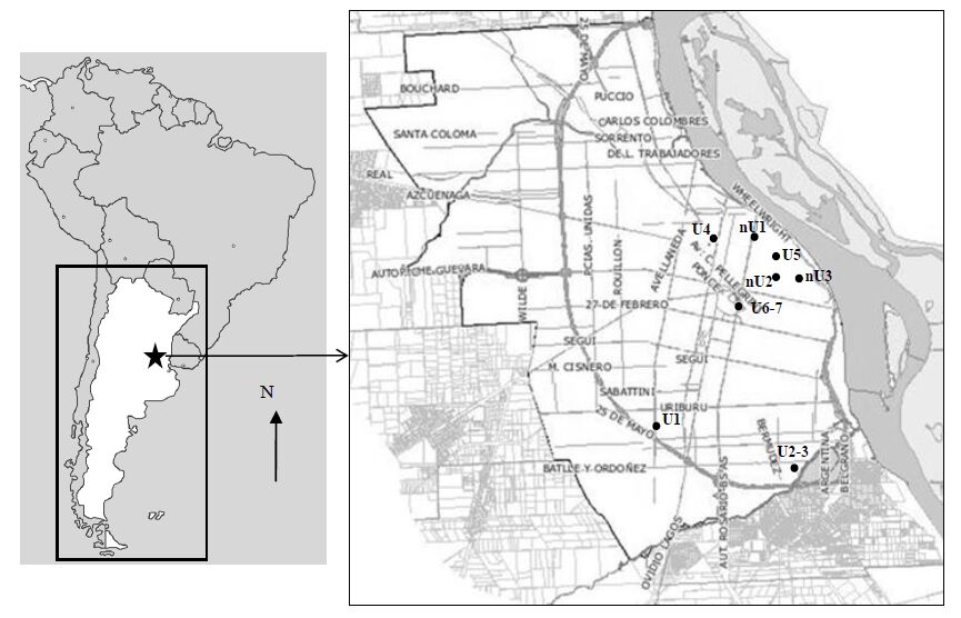
[29] | Municipalidad de Rosario (2014) Available from: http://www.rosario.gov.ar/sitio/caracteristicas/geografica_limites.jsp. |
[30] | Servicio Meteorológico Nacional (2014) Available from: http://www.smn.gov.ar/serviciosclimaticos/?mod=turismo&id=7&provincia=Santa%20Fe&ciudad=Rosario. |
[31] | Municipalidad de Rosario (2015) Available from: http://www.rosario.gov.ar/sitio/desarrollo_social/empleo/programa_au.jsp. |
[32] | Castellani A, Skolnik M (2011) “Devaluacionistas” y “dolarizadores”. La construcción social de las alternativas propuestas por los sectores dominantes ante la crisis de la Convertibilidad. Argentina 1999-2001. Doc Invest Soc 18: 1-21. |
[33] |
Potchter O, Cohen P, Bitan A (2006) Climatic behaviour of various urban parks during hot and humid summer in the Mediterranean city of Tel Aviv, Israel. Int J Climatol 26: 1695-1711. doi: 10.1002/joc.1330
![]() |
[34] |
Vardoulakis E, Karamanis D, Fotiadi D, et al. (2013) The urban heat island effect in a small Mediterranean city of high summer temperatures and cooling energy demands. Solar Energy 94:128-144. doi: 10.1016/j.solener.2013.04.016
![]() |
[35] | Peck JE (2010) Multivariate analysis for community ecologists: step-by-step using PC-ORD. MjM Software Design, US. |
[36] | Szokolay SV (2004) Introduction to architectural science the basis of sustainable design. Oxford. Elsevier, pp 360. |
[37] | Di Rienzo JA, Casanoves F, Balzarini MG, et al. (2008) InfoStat, versión 2008. Córdoba. Universidad Nacional de Córdoba, Argentina. |
[38] | Barros V, Vera C, Agosta E, et al. (2015) Cambio climático en Argentina; tendencias y proyecciones. Tercera Comunicación Nacional a la Convención Marco de las Naciones Unidas sobre el Cambio Climático. Available from: http://www.ambiente.gov.ar/?idarticulo=13291 |
[39] | IPCC (2000) Emission scenarios, a special report of working group III of the intergovernmental on climate change. Nakicenovic N. Coordinating Lead Author. Cambridge University Press, Cambridge, pp 570. |
[40] | Núñez M, Solman S, Cabré MF (2009) Regional climate change experiments over southern South America. II: Climate change scenarios in the late twenty-first century. Clim Dynam 32: 1081-1095. |
[41] | Camilloni I (2014) Isla urbana de calor. Atlas ambiental de Buenos Aires. Available from: http://www.atlasdebuenosaires.gov.ar/aaba/index.php?option=com_content&task=view&id=416&Itemid=207&lang=es. |
[42] | Oke TR (1982) The energetic basis of the urban heal island. Q J Roy Meteor Soc 108: 1-24. |
[43] |
Hardoy J, Ruete R (2013) Incorporating climate change adaptation into planning for a liveable city in Rosario, Argentina. Environ Urban 25: 339-360. doi: 10.1177/0956247813493232
![]() |
1. | Ming Chen, Lale Asik, Angela Peace, Stoichiometric knife-edge model on discrete time scale, 2019, 2019, 1687-1847, 10.1186/s13662-019-2468-7 | |
2. | Lale Asik, Jackson Kulik, Kevin R. Long, Angela Peace, Seasonal Variation of Nutrient Loading in a Stoichiometric Producer–Consumer System, 2019, 81, 0092-8240, 2768, 10.1007/s11538-019-00629-6 | |
3. | Md. Nazmul Hassan, Lale Asik, Jackson Kulik, K.R. Long, Angela Peace, Environmental seasonality on predator–prey systems under nutrient and toxicant constraints, 2019, 480, 00225193, 71, 10.1016/j.jtbi.2019.08.001 |