Revealing the biotechnological potential of Delftia sp. JD2 by a genomic approach

María A. Morel; Andrés Iriarte; Eugenio Jara; Héctor Musto; Susana Castro-Sowinski; María A. Morel; Andrés Iriarte; Eugenio Jara; Héctor Musto; Susana Castro-Sowinski

doi:10.3934/bioeng.2016.2.156

AIMS Bioengineering

2016, Volume 3, Issue 2: 156-175. doi: 10.3934/bioeng.2016.2.156

Previous Article Next Article

Research article Topical Sections

Revealing the biotechnological potential of Delftia sp. JD2 by a genomic approach

1.
Unidad Microbiología Molecular, Instituto de Investigaciones Biológicas Clemente Estable (IIBCE). Av Italia 3318, 11600, Montevideo, Uruguay
2.
Dpto de Bioquímica y Genómica Microbiana and Dpto de Genómica (IIBCE), Av. Italia 3318, 11600, Montevideo, Uruguay
3.
Dpto de Desarrollo Biotecnológico, Instituto de Higiene, Facultad de Medicina, Universidad de la República (UdelaR), Av. Gral. Flores 2125, 11800, Montevideo, Uruguay
4.
Organización y Evolución del Genoma, Facultad de Ciencias, UdelaR, Iguá 4225, 11400, Montevideo, Uruguay
5.
Sección Bioquímica y Biología Molecular, Facultad de Ciencias, UdelaR, Iguá 4225, 11400, Montevideo, Uruguay

Received: 07 March 2016 Accepted: 12 April 2016 Published: 14 April 2016

Delftia sp. JD2 is a chromium-resistant bacterium that reduces Cr(VI) to Cr(III), accumulates Pb(II), produces the phytohormone indole-3-acetic acid and siderophores, and increases the plant growth performance of rhizobia in co-inoculation experiments. We aimed to analyze the biotechnological potential of JD2 using a genomic approach. JD2 has a genome of 6.76Mb, with 6,051 predicted protein coding sequences and 93 RNA genes (tRNA and rRNA). The indole-acetamide pathway was identified as responsible for the synthesis of indole-3-acetic acid. The genetic information involved in chromium resistance (the gene cluster, chrBACF,) was found. At least 40 putative genes encoding for TonB-dependent receptors, probably involved in the utilization of siderophores and biopolymers, and genes for the synthesis, maturation, exportation and uptake of pyoverdine, and acquisition of Fe-pyochelin and Fe-enterobactin were also identified. The information also suggests that JD2 produce polyhydroxybutyrate, a carbon reserve polymer commonly used for manufacturing petrochemical free bioplastics. In addition, JD2 may degrade lignin-derived aromatic compounds to 2-pyrone-4,6-dicarboxylate, a molecule used in the bio-based polymer industry. Finally, a comparative genomic analysis of JD2, Delftia sp. Cs1-4 and Delftia acidovorans SPH-1 is also discussed. The present work provides insights into the physiology and genetics of a microorganism with many potential uses in biotechnology.
- Delftia,
- plant-growth promotion,
- bioremediation,
- comparative genomic,
- plant-microbe interaction
Citation: María A. Morel, Andrés Iriarte, Eugenio Jara, Héctor Musto, Susana Castro-Sowinski. Revealing the biotechnological potential of Delftia sp. JD2 by a genomic approach[J]. AIMS Bioengineering, 2016, 3(2): 156-175. doi: 10.3934/bioeng.2016.2.156

Related Papers:

Abstract

Delftia sp. JD2 is a chromium-resistant bacterium that reduces Cr(VI) to Cr(III), accumulates Pb(II), produces the phytohormone indole-3-acetic acid and siderophores, and increases the plant growth performance of rhizobia in co-inoculation experiments. We aimed to analyze the biotechnological potential of JD2 using a genomic approach. JD2 has a genome of 6.76Mb, with 6,051 predicted protein coding sequences and 93 RNA genes (tRNA and rRNA). The indole-acetamide pathway was identified as responsible for the synthesis of indole-3-acetic acid. The genetic information involved in chromium resistance (the gene cluster, chrBACF,) was found. At least 40 putative genes encoding for TonB-dependent receptors, probably involved in the utilization of siderophores and biopolymers, and genes for the synthesis, maturation, exportation and uptake of pyoverdine, and acquisition of Fe-pyochelin and Fe-enterobactin were also identified. The information also suggests that JD2 produce polyhydroxybutyrate, a carbon reserve polymer commonly used for manufacturing petrochemical free bioplastics. In addition, JD2 may degrade lignin-derived aromatic compounds to 2-pyrone-4,6-dicarboxylate, a molecule used in the bio-based polymer industry. Finally, a comparative genomic analysis of JD2, Delftia sp. Cs1-4 and Delftia acidovorans SPH-1 is also discussed. The present work provides insights into the physiology and genetics of a microorganism with many potential uses in biotechnology.

References

[1]	De Gusseme B, Vanhaecke L, Verstraete W, et al. (2011) Degradation of acetaminophen by Delftia tsuruhatensis and Pseudomonas aeruginosa in a membrane bioreactor. Water Res 45: 1829–1837. doi: 10.1016/j.watres.2010.11.040
[2]	Juárez-Jiménez B, Manzanera M, Rodelas B, et al. (2010) Metabolic characterization of a strain (BM90) of Delftia tsuruhatensis showing highly diversified capacity to degrade low molecular weight phenols. Biodegradation 21: 475–489. doi: 10.1007/s10532-009-9317-4
[3]	Leibeling S, Schmidt F, Jehmlich N, et al. (2010) Declining capacity of starving Delftia acidovorans MC1 to degrade phenoxypropionate herbicides correlates with oxidative modification of the initial enzyme. Environ Sci Technol 44: 3793–3799. doi: 10.1021/es903619j
[4]	Morel MA, Ubalde MC, Braña V, et al. (2011) Delftia sp. JD2: a potential Cr (VI)-reducing agent with plant growth-promoting activity. Arch Microbiol 193: 63–68.
[5]	Paulin MM, Nicolaisen MH, Sørensen J (2010) Abundance and expression of enantioselective rdpA and sdpA dioxygenase genes during degradation of the racemic herbicide (R, S)-2-(2, 4-dichlorophenoxy) propionate in soil. Appl Environ Microbiol 76: 2873–2883. doi: 10.1128/AEM.02270-09
[6]	Vacca DJ, Bleam WF, Hickey WJ (2005) Isolation of soil bacteria adapted to degrade humic acid-sorbed phenanthrene. Appl Environ Microbiol 71: 3797–3805. doi: 10.1128/AEM.71.7.3797-3805.2005
[7]	Yan H, Yang X, Chen J, et al. (2011) Synergistic removal of aniline by carbon nanotubes and the enzymes of Delftia sp. XYJ6. J Environ Sci 23: 1165–1170. doi: 10.1016/S1001-0742(10)60531-1
[8]	Zhang LL, He D, Chen JM, et al. (2010). Biodegradation of 2-chloroaniline, 3-chloroaniline, and 4-chloroaniline by a novel strain Delftia tsuruhatensis H1. J Hazard Mater 179: 875–882. doi: 10.1016/j.jhazmat.2010.03.086
[9]	Wu W, Huang H, Ling Z, et al. (2015). Genome sequencing reveals mechanisms for heavy metal resistance and polycyclic aromatic hydrocarbon degradation in Delftia lacustris strain LZ-C. Ecotoxicology 25: 234–247.
[10]	Han J, Sun L, Dong X, et al. (2005) Characterization of a novel plant growth-promoting bacteria strain Delftia tsuruhatensis HR4 both as a diazotroph and a potential biocontrol agent against various plant pathogens. Syst Appl Microbiol 28: 66–76. doi: 10.1016/j.syapm.2004.09.003
[11]	Morel MA, Cagide C, Minteguiaga MA, et al. (2015) The pattern of secreted molecules during the co-inoculation of alfalfa plants with Sinorhizobium meliloti and Delftia sp. strain JD2: an interaction that improves plant yield. Mol Plant-Microbe Int 28: 134–142.
[12]	Ubalde MC, Braña V, Sueiro F, et al. (2012) The versatility of Delftia sp. isolates as tools for bioremediation and biofertilization technologies. Curr Microbiol 64: 597–603.
[13]	Camargo CH, Ferreira AM, Javaroni E, et al. (2014) Microbiological characterization of Delftia acidovorans clinical isolates from patients in an intensive care unit in Brazil . Diagn Microbiol Infect Dis 80: 330–333. doi: 10.1016/j.diagmicrobio.2014.09.001
[14]	Mahmood S, Taylor KE, Overman TL, et al. (2012) Acute infective endocarditis caused by Delftia acidovorans, a rare pathogen complicating intravenous drug use. J Clin Microbiol 50: 3799–3800. doi: 10.1128/JCM.00553-12
[15]	Morel MA, Castro-Sowinski S, (2013) The complex molecular signaling network in microbe-plant interaction. In: Arora N (ed) Plant microbe symbiosis: Fundamentals and Advances. Springer India , pp. 169–199.
[16]	Morel MA, Ubalde MC, Olivera-Bravo S, et al. (2009) Cellular and biochemical response to Cr (VI) in Stenotrophomonas sp. FEMS Microbiol Lett 291: 162–168. doi: 10.1111/j.1574-6968.2008.01444.x
[17]	Sambrook J, Frietsch EF, Maniatis T, (1989) Molecular cloning: A LaboratoryManual, 2nd Edn. Cold Spring Harbor Laboratory, Cold Spring Harbor, New York.
[18]	Bankevich A, Nurk S, Antipov D, et al. (2012) SPAdes: a new genome assembly algorithm and its applications to single-cell sequencing. J Comput Biol 19: 455–477. doi: 10.1089/cmb.2012.0021
[19]	Assefa S, Keane TM, Otto TD, et al. (2009) ABACAS: algorithm-based automatic contiguation of assembled sequences. Bioinformatics 25: 1968–1969. doi: 10.1093/bioinformatics/btp347
[20]	Schleheck D, Knepper TP, Fischer K, et al. (2004) Mineralization of individual congeners of linear alkylbenzenesulfonate (LAS) by defined pairs of heterotrophic bacteria. Appl Environ Microbiol 70: 4053–4063. doi: 10.1128/AEM.70.7.4053-4063.2004
[21]	Aziz RK, Bartels D, Best AA, et al. (2008) The RAST Server: rapid annotations using subsystems technology. BMC Genomics 9: 75. doi: 10.1186/1471-2164-9-75
[22]	Overbeek R, Begley T, Butler RM, et al. (2005) The subsystems approach to genome annotation and its use in the project to annotate 1000 genomes. Nucl Acid Res 33: 5691–5702. doi: 10.1093/nar/gki866
[23]	Marchler-Bauer A, Lu S, Anderson JB, et al. (2011) CDD: a Conserved Domain Database for the functional annotation of proteins. Nucl Acid Res 39: D225–229. doi: 10.1093/nar/gkq1189
[24]	Li L, Stoeckert CJ Jr, Roos DS (2003) OrthoMCL: identification of ortholog groups for eukaryotic genomes. Genome Res 13: 2178–89. doi: 10.1101/gr.1224503
[25]	Contreras-Moreira B, Vinuesa P (2013) GET_HOMOLOGUES, a versatile software package for scalable and robust microbial pangenome analysis. Appl Environ Microbiol 79: 7696–7701. doi: 10.1128/AEM.02411-13
[26]	Sievers F, Wilm A, Dineen DG, et al. (2011) Fast, scalable generation of high-quality protein multiple sequence alignments using Clustal Omega. Mol Syst Biol 7: 539.
[27]	Guindon S, Gascuel O (2003) PhyML: A simple, fast and accurate algorithm to estimate large phylogenies by maximum likelihood. Syst Biol 52: 696–704. doi: 10.1080/10635150390235520
[28]	Guindon S, Dufayard JF, Lefort V (2010) New algorithms and methods to estimate maximum-likelihood phylogenies: assessing the performance of PhyML 3.0. Syst Biol 59: 307–321. doi: 10.1093/sysbio/syq010
[29]	Sukumaran J, Holder MT (2010) DendroPy: a Python library for phylogenetic computing. Bioinformatics 26: 1569–1571. doi: 10.1093/bioinformatics/btq228
[30]	Tamura K, Stecher G, Peterson D, et al. (2013) MEGA6: Molecular Evolutionary Genetics Analysis version 6.0. Mol Biol Evol 30: 2725–2729. doi: 10.1093/molbev/mst197
[31]	Goris J, Konstantinidis KT, Klappenbach JA, et al. (2007) DNA-DNA hybridization values and their relationship to whole-genome sequence similarities. Int J Syst Evol Microbiol 57: 81–91. doi: 10.1099/ijs.0.64483-0
[32]	Hulsen T, de Vlieg J, Alkema W (2008) BioVenn - a web application for the comparison and visualization of biological lists using area-proportional Venn diagrams. BMC Genomic 9: 488. doi: 10.1186/1471-2164-9-488
[33]	Noinaj N, Guillier M, Barnard TJ, et al. (2010) TonB-dependent transporters: regulation, structure, and function. Ann Rev Microbiol 64: 43–60. doi: 10.1146/annurev.micro.112408.134247
[34]	Hara H, Masai E, Katayama Y, et al. (2000) The 4-oxalomesaconate hydratase gene, involved in the protocatechuate 4, 5-cleavage pathway, is essential to vanillate and syringate degradation in Sphingomonas paucimobilis SYK-6. J Bacteriol 182: 6950–6957. doi: 10.1128/JB.182.24.6950-6957.2000
[35]	Providenti MA, Mampel J, MacSween S, et al. (2001) Comamonas testosteroni BR6020 possesses a single genetic locus for extradiol cleavage of protocatechuate. Microbiol 147: 2157–2167. doi: 10.1099/00221287-147-8-2157
[36]	Masai E, Katayama Y, Fukuda M (2007) Genetic and biochemical investigations on bacterial catabolic pathways for lignin-derived aromatic compounds. Biosci Biotechnol Biochem 71: 1–15. doi: 10.1271/bbb.60437
[37]	Baldoma L, Aguilar J (1988) Metabolism of L-fucose and L-rhamnose in Escherichia coli: aerobic-anaerobic regulation of L-lactaldehyde dissimilation. J Bacteriol 170: 416–421.
[38]	Chan JY, Nwokoro NA, Schachter H (1979) L-fucose metabolism in mammals. The conversion of L-fucose to two moles of L-lactate, of L-galactose to L-lactose and glycerate, and of D-arabinose to L-lactate and glycollate. J Biol Chem 254: 7060–7068.
[39]	Matsusaki H, Manji S, Taguchi K, et al. (1998) Cloning and molecular analysis of the poly (3-hydroxybutyrate) and poly (3-hydroxybutyrate-co-3-hydroxyalkanoate) biosynthesis genes in Pseudomonas sp. strain 61-3. J Bacteriol 180: 6459–6467.
[40]	Tirapelle EF, Müller-Santos M, Tadra-Sfeir MZ, et al. (2013) Identification of proteins associated with polyhydroxybutyrate granules from Herbaspirillum seropedicae SmR1 - Old partners, New players. PloS ONE 8: e75066. doi: 10.1371/journal.pone.0075066
[41]	Davenport KW, Daligault HE, Minogue TD, et al. (2014) Draft genome assembly of Delftia acidovorans type strain 2167. Genome Announc 2: e00917–14.
[42]	Shetty AR, de GAnnes V, Obi CC, Lucas S, et al. (2015) Complete genome sequencing of the phananthrene-degrading soil bacterium Delftia acidovorans Cs1-4. Stand Genomic Sci 10: 55. doi: 10.1186/s40793-015-0041-x
[43]	Hou Q, Wang C, Guo H, et al. (2015). Draft genome sequence fo Delftia tsuruhatensis MTQ3, a strain of plant growth-promoting rhizobacterium with antimicrobial activity. Genome Announc 3: e00822–15.
[44]	Leadbetter JR, Greenberg EP (2000) Metabolism of acyl-homoserine lactone quorum-sensing signals by Variovorax paradoxus. J Bacteriol 182: 6921–6926. doi: 10.1128/JB.182.24.6921-6926.2000
[45]	Weelink SAB, Tan NCB, ten Broeke H, et al. (2008) Isolation and characterization of Alicycliphilus denitrificans strain BC, which grows on benzene with chlorate as the electron acceptor. Appl Environ Microbiol 74: 6672–6681. doi: 10.1128/AEM.00835-08
[46]	Kim M, Oh HS, Park SC, et al. (2014) Towards a taxonomic coherence between average nucleotide identity and 16S rRNA gene sequence similarity for species demarcation of prokaryotes. Int J Syst Evol Microbiol 64: 346–351. doi: 10.1099/ijs.0.059774-0
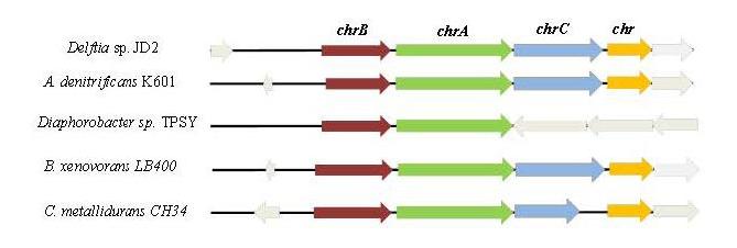
[47]	Branco R, Chung AP, Johnston T, et al. (2008) The chromate-inducible chrBACF operon from the transposable element TnOtChr confers resistance to chromium (VI) and superoxide. J Bacteriol 190: 6996–7003. doi: 10.1128/JB.00289-08
[48]	Branco R, Morais PV (2013). Identification and characterization of the transcriptional regulator ChrB in the chromate resistance determinant of Ochrobactrum tritici 5bvl1. PLoS ONE 8: e77987.
[49]	Morais PV, Branco R, Francisco R (2011) Chromium resistance strategies and toxicity: what makes Ochrobactrum tritici 5bvl1 a strain highly resistant. Biometals 24: 401–410. doi: 10.1007/s10534-011-9446-1
[50]	Juhnke S, Peitzsch N, Hübener N, et al. (2002) New genes involved in chromate resistance in Ralstonia metallidurans strain CH34. Arch Microbiol 179: 15–25. doi: 10.1007/s00203-002-0492-5
[51]	Liu KJ, Shi X, Dalal NS (1997) Synthesis of Cr(IV) GSH, its identification and its free hydroxal radical generation: a model compound for Cr(VI) carcinogenicity. Biochem Biophys Res Comm 235: 54–58. doi: 10.1006/bbrc.1997.6277
[52]	Nies A, Nies DH, Silver S. (1990) Nucleotide sequence and expression of a plasmid-encoded chromate resistance determinant from Alcaligenes eutrophus. J Biol Chem 265: 5648–5653.
[53]	Yun J-H, Cho Y-J, Chun J, et al. (2014) Genome sequence of the chromate-resistant bacterium Leucobacter salsicius type strain M1-8T. Stand Genomic Sci 9: 495–504.
[54]	Mahillon J, Michael C (1998) Insertion sequences. Microbiol Mol Biol Rev 62: 725–774.
[55]	Spaepen S, Vanderleyden J, Remans R (2007) Indole-3-acetic acid in microbial and microorganism-plant signaling. FEMS Microbiol Rev 31: 425–448. doi: 10.1111/j.1574-6976.2007.00072.x
[56]	Lambrecht M, Okon Y, Broek AV, et al. (2000) Indole-3-acetic acid: a reciprocal signalling molecule in bacteria–plant interactions. Trends Microbiol 8: 298–300. doi: 10.1016/S0966-842X(00)01732-7
[57]	Duan J, Jian W, Cheng Z, et al. (2013) The complete genome sequence of the plant growth-promoting bacterium Pseudomonas sp. UW4. PLoS ONE 8: e58640. doi: 10.1371/journal.pone.0058640
[58]	Sant´Anna FH, Almeida LGP, Cecagno R, et al. (2011) Genomic insights into the versatility of the plant growth-promoting bacterium Azospirillum amazonense. BMC Genomics 12: 409. doi: 10.1186/1471-2164-12-409
[59]	Spaepen S, Vanderleyden J (2011) Auxin and plant-microbe interactions. Cold Spring Harb Perspect Biol 3: a001438.
[60]	Merino E, Jensen RA, Yanofsky C (2008) Evolution of bacterial trp operons and their regulation. Curr Opin Microbiol 11: 78–86. doi: 10.1016/j.mib.2008.02.005
[61]	Wood H, Roshick C, McClarty G (2004) Tryptophan recycling is responsible for the interferon -γ resistance of Chlamydia psittaci GPIC in indoleamine dioxygenase-expressing host cells. Mol Microbiol 52: 903–916. doi: 10.1111/j.1365-2958.2004.04029.x
[62]	Merkl R (2007) Modelling the evolution of the archaeal tryptophan synthase. BMC Evol Biol 7: 59. doi: 10.1186/1471-2148-7-59
[63]	Olekhnovich I, Gussin GN (2001) Effects of mutations in the Pseudomonas putida miaA gene: regulation of the trpE and trpGDC operons in P. putida by attenuation. J Bacteriol 183: 3256–3260.
[64]	Hibbing ME, Fuqua C, Parsek MR, et al. (2010) Bacterial competition: surviving and thriving in the microbial jungle. Nat Rev Microbiol 8: 15–25. doi: 10.1038/nrmicro2259
[65]	Compant S, Duffy B, Nowak J, et al. (2005) Use of plant growth-promoting bacteria for biocontrol of plant diseases: principles, mechanisms of action, and future prospects. Appl Environ Microbiol 7: 4951–4959.
[66]	Dimkpa CO, Svatoš A, Dabrowska P, et al. (2008) Involvement of siderophores in the reduction of metal-induced inhibition of auxin synthesis in Streptomyces spp. Chemosphere 74: 19–25. doi: 10.1016/j.chemosphere.2008.09.079
[67]	Hussein KA, Joo JH (2014) Potential of siderophore production by bacteria isolated from heavy metal: polluted and rhizosphere soils. Curr Microbiol 68: 717–723. doi: 10.1007/s00284-014-0530-y
[68]	Rajkumar M, Ae N, Prasad MNV, et al. (2010) Potential of siderophore-producing bacteria for improving heavy metal phytoextraction. Trends Biotech 28: 142–149. doi: 10.1016/j.tibtech.2009.12.002
[69]	Schalk IJ, Guillon L (2013) Pyoverdine biosynthesis and secretion in Pseudomonas aeruginosa: implications for metal homeostasis. Environ Microbiol 15: 1661–1673. doi: 10.1111/1462-2920.12013
[70]	Jørgensen NO, Brandt KK, Nybroe O, et al. (2009) Delftia lacustris sp. nov., a peptidoglycan-degrading bacterium from fresh water, and emended description of Delftia tsuruhatensis as a peptidoglycan-degrading bacterium. Int J Syst Evol Microbiol 59: 2195–2199.
[71]	Prasannakumar SP, Gowtham HG, Hariprasad P, et al. (2015) Delftia tsuruhatensis WGR–UOM–BT1, a novel rhizobacterium with PGPR properties from Rauwolfia serpentina (L.) Benth. ex Kurz also suppresses fungal phytopathogens by producing a new antibiotic-AMTM. Lett Appl Microbiol 61: 460–468.
[72]	Bugg TDH, Ahmad M, Hardiman EM, et al. (2011). The emerging role for bacteria in lignin degradation and bio-product formation. Curr Opin Biotechnol 22(3): 394–400.
[73]	Vicuña R, Gonzalez B, Mozuch MD, et al. (1987) Metabolism of lignin model compounds of the arylglycerol-β-aryl ether type by Pseudomonas acidovorans D3. Appl Environ Microbiol 53: 2605–2609.
[74]	Otsuka Y, Nakamura M, Shigehara K, et al. (2006) Efficient production of 2-pyrone 4, 6-dicarboxylic acid as a novel polymer-based material from protocatechuate by microbial function. Appl Microbiol Biotech 71: 608–614. doi: 10.1007/s00253-005-0203-7
[75]	Hwang HJ, Lee SY, Kim SM, et al. (2011) Fermentation of seaweed sugars by Lactobacillus species and the potential of seaweed as a biomass feedstock. Biotechnol Bioprocess Eng 16: 1231–1239. doi: 10.1007/s12257-011-0278-1
[76]	John RP, Anisha GS, Nampoothiri KM, et al. (2009) Direct lactic acid fermentation: focus on simultaneous saccharification and lactic acid production. Biotechnol Adv 27: 145–152. doi: 10.1016/j.biotechadv.2008.10.004
[77]	Gumel AM, Annuar MSM, Heidelberg T (2012) Effects of carbon substrates on biodegradable polymer composition and stability produced by Delftia tsuruhatensis Bet002 isolated from palm oil mill effluent. Polym Degrad Stabil 97: 1224–1231. doi: 10.1016/j.polymdegradstab.2012.05.041
[78]	Hsieh WC, Wada Y, Chang CP (2009) Fermentation, biodegradation and tensile strength of poly (3-hydroxybutyrate-co-4-hydroxybutyrate) synthesized by Delftia acidovorans. J Taiwan Inst Chem Eng 40: 143–147. doi: 10.1016/j.jtice.2008.11.004
[79]	Loo CY, Sudesh K (2007) Biosynthesis and native granule characteristics of poly (3-hydroxybutyrate-co-3-hydroxyvalerate) in Delftia acidovorans. Int J Biol Macromol 40: 466–471. doi: 10.1016/j.ijbiomac.2006.11.003
[80]	Tsuge T, Takase K, Taguchi S, et al. (2004) An extra large insertion in the polyhydroxyalkanoate synthase from Delftia acidovorans DS-17: its deletion effects and relation to cellular proteolysis. FEMS Microbiol Lett 231: 77–83. doi: 10.1016/S0378-1097(03)00930-3

Reader Comments

Your name:*

Email:*
© 2016 the Author(s), licensee AIMS Press. This is an open access article distributed under the terms of the Creative Commons Attribution License (http://creativecommons.org/licenses/by/4.0)