The composition of soils in aquifers is typically not homogeneous, and soil layers may be cracked or displaced due to geological activities. This heterogeneity in soil distribution within aquifers affects groundwater flow and water level variations. In the present study, we established a two-dimensional (2D) mathematical model that considers the influence of surface recharge on groundwater flow in heterogeneous sloping aquifers. By considering temporal variations in surface recharge, slope angle and aquifer heterogeneity, the simulated results are expected to better reflect real conditions in natural aquifers. The effects of aquifer heterogeneity on groundwater flow and water levels are particularly significant in sloping aquifers. The study's findings indicate that even when the soil composition remains constant, variations in groundwater level and flow may be considerable, depending on factors such as soil alignment, slope angle of the aquifer's base layer and the direction of water flow.
Citation: Ming-Chang Wu, Ping-Cheng Hsieh. Influence of nonuniform recharge on groundwater flow in heterogeneous aquifers[J]. AIMS Mathematics, 2023, 8(12): 30120-30141. doi: 10.3934/math.20231540
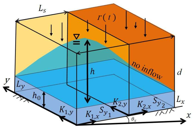
The composition of soils in aquifers is typically not homogeneous, and soil layers may be cracked or displaced due to geological activities. This heterogeneity in soil distribution within aquifers affects groundwater flow and water level variations. In the present study, we established a two-dimensional (2D) mathematical model that considers the influence of surface recharge on groundwater flow in heterogeneous sloping aquifers. By considering temporal variations in surface recharge, slope angle and aquifer heterogeneity, the simulated results are expected to better reflect real conditions in natural aquifers. The effects of aquifer heterogeneity on groundwater flow and water levels are particularly significant in sloping aquifers. The study's findings indicate that even when the soil composition remains constant, variations in groundwater level and flow may be considerable, depending on factors such as soil alignment, slope angle of the aquifer's base layer and the direction of water flow.

| [1] |
M. Hartmann, S. Kullmann, H. Keller, Wastewater treatment with heterogeneous Fenton-type catalysts based on porous materials, J. Mater. Chem., 20 (2010), 9002–9017. https://doi.org/10.1039/C0JM00577K doi: 10.1039/C0JM00577K

|
| [2] |
F. A. Montalto, T. S. Steenhuis, J. Y. Parlange, The hydrology of Piermont Marsh, a reference for tidal marsh restoration in the Hudson river estuary, New York, J. Hydrol., 316 (2006), 108–128. https://doi.org/10.1016/j.jhydrol.2005.03.043 doi: 10.1016/j.jhydrol.2005.03.043
|
| [3] |
E. A. Sudicky, P. S. Huyakorn, Contaminant migration in imperfectly known heterogeneous groundwater systems, Rev. Geophys., 29 (1991), 240–253. https://doi.org/10.1002/rog.1991.29.s1.240 doi: 10.1002/rog.1991.29.s1.240
|
| [4] |
S. E. Serrano, Analytical solutions of the nonlinear groundwater flow equation in unconfined aquifers and the effect of heterogeneity, Water Resour. Res., 31 (1995), 2733–2742. https://doi.org/10.1029/95WR02038 doi: 10.1029/95WR02038
|
| [5] |
J. Cao, P. K. Kitanidis, Adaptive-grid simulation of groundwater flow in heterogeneous aquifers, Adv. Water Resour., 22 (1999), 681–696. https://doi.org/10.1016/S0309-1708(98)00047-5 doi: 10.1016/S0309-1708(98)00047-5
|
| [6] |
T. Scheibe, S. Yabusaki, Scaling of flow and transport behavior in heterogeneous groundwater systems, Adv. Water Resour., 22 (1998), 223–238. https://doi.org/10.1016/S0309-1708(98)00014-1 doi: 10.1016/S0309-1708(98)00014-1
|
| [7] |
C. L. Winter, D. M. Tartakovsky, Groundwater flow in heterogeneous composite aquifers, Water Resour. Res., 38 (2002), 23-1. https://doi.org/10.1029/2001WR000450 doi: 10.1029/2001WR000450
|
| [8] |
C. W. Beckwith, A. J. Baird, A. L. Heathwaite, Anisotropy and depth‐related heterogeneity of hydraulic conductivity in a bog peat. Ⅱ: modelling the effects on groundwater flow, Hydrol. Process., 17 (2003), 103–113. https://doi.org/10.1002/hyp.1116 doi: 10.1002/hyp.1116
|
| [9] |
K. Hemker, M. Bakker, Analytical solutions for whirling groundwater flow in two-dimensional heterogeneous anisotropic aquifers, Water Resour. Res., 42 (2006), 55–65. https://doi.org/10.1029/2006WR004901 doi: 10.1029/2006WR004901
|
| [10] |
M. Fahs, T. Graf, T. V. Tran, B. Ataie-Ashtiani, C. T. Simmons, A. Younes, Study of the effect of thermal dispersion on internal natural convection in porous media using Fourier series, Transport Porous Med., 131 (2000), 537–568. https://doi.org/10.1007/s11242-019-01356-1 doi: 10.1007/s11242-019-01356-1
|
| [11] |
K. Srivastava, S. E. Serrano, Uncertainty analysis of linear and nonlinear groundwater flow in a heterogeneous aquifer, J. Hydrol. Eng., 12 (2007), 306–318. https://doi.org/10.1061/(ASCE)1084-0699(2007)12:3(306) doi: 10.1061/(ASCE)1084-0699(2007)12:3(306)
|
| [12] |
S. K. Das, S. Jai Ganesh, T. S. Lundström, Modeling of a groundwater mound in a two-dimensional heterogeneous unconfined aquifer in response to precipitation recharge, J. Hydrol. Eng., 20 (2015), 04014081-1-12. https://doi.org/10.1061/(ASCE)HE.1943-5584.0001071 doi: 10.1061/(ASCE)HE.1943-5584.0001071
|
| [13] |
M. C. Wu, P. C. Hsieh, Improved solutions to the linearized Boussinesq equation with temporally varied rainfall recharge for a sloping aquifer, Water, 11 (2019), 826. https://doi.org/10.3390/w11040826 doi: 10.3390/w11040826
|
| [14] |
K. N. Moutsopoulos, J. N. Papaspyros, M. Fahs, Approximate solutions for flows in unconfined double porosity aquifers, J. Hydrol., (2022), 615. https://doi.org/10.1016/j.jhydrol.2022.128679 doi: 10.1016/j.jhydrol.2022.128679
|
| [15] |
N. Samani, M. M. Sedghi, Semi-analytical solutions of groundwater flow in multi-zone (patchy) wedge-shaped aquifers, Adv. Water Resour., 77 (2015), 1–16. https://doi.org/10.1016/j.advwatres.2015.01.003 doi: 10.1016/j.advwatres.2015.01.003
|
| [16] |
X. Liang, Y. K. Zhang, K. Schilling, Effect of heterogeneity on spatiotemporal variations of groundwater level in a bounded unconfined aquifer, Stoch. Env. Res. Risk A., 30 (2016), 1–8. https://doi.org/10.1007/s00477-014-0990-4 doi: 10.1007/s00477-014-0990-4
|
| [17] |
X. Liang, H. Zhan, K. Schilling, Spatiotemporal responses of groundwater flow and aquifer‐river exchanges to flood events, Water Resour. Res., 54 (2018), 1513–1532. https://doi.org/10.1002/2017WR022046 doi: 10.1002/2017WR022046
|
| [18] |
J. F. Águila, J. Samper, B. Pisani, Parametric and numerical analysis of the estimation of groundwater recharge from water-table fluctuations in heterogeneous unconfined aquifers, Hydrogeol. J., 27 (2019), 1309–1328. https://doi.org/10.1007/s10040-018-1908-x doi: 10.1007/s10040-018-1908-x
|
| [19] |
E. Akylas, A. D. Koussis, Response of sloping unconfined aquifer to stage changes in adjacent stream. Ⅰ. Theoretical analysis and derivation of system response functions, J. Hydrol., 338 (2007), 85–95. https://doi.org/10.1016/j.jhydrol.2007.02.021 doi: 10.1016/j.jhydrol.2007.02.021
|
| [20] |
A. D. Koussis, E. Akylas, K. Mazi, Response of sloping unconfined aquifer to stage changes in adjacent stream: Ⅱ. Applications, J. Hydrol., 338 (2007), 73–84. https://doi.org/10.1016/j.jhydrol.2007.02.030 doi: 10.1016/j.jhydrol.2007.02.030
|
| [21] |
M. C. Wu, P. C. Hsieh, Variation of groundwater flow caused by any spatiotemporally varied recharge, Water, 12 (2020), 287. https://doi.org/10.3390/w12010287 doi: 10.3390/w12010287
|
| [22] |
J. Zhang, X. Liang, Y. K. Zhang, X. Chen, E. Ma, K. Schilling, Groundwater responses to recharge and flood in riparian zones of layered aquifers: An analytical model, J. Hydrol., (2022), 614. https://doi.org/10.1016/j.jhydrol.2022.128547 doi: 10.1016/j.jhydrol.2022.128547
|
| [23] |
W. Brutsaert, The unit response of groundwater outflow from a hillslope, Water Resour. Res., 30 (1994), 2759–2763. https://doi.org/10.1029/94WR01396 doi: 10.1029/94WR01396
|
| [24] |
M. A. Marino, Water-table fluctuation in semipervious stream-unconfined aquifer systems, J. Hydrol., 19 (1973), 43–52. https://doi.org/10.1016/0022-1694(73)90092-9 doi: 10.1016/0022-1694(73)90092-9
|


Figures(9) / Tables(1)

Ming-Chang Wu, Ping-Cheng Hsieh. Influence of nonuniform recharge on groundwater flow in heterogeneous aquifers[J]. AIMS Mathematics, 2023, 8(12): 30120-30141. doi: 10.3934/math.20231540


 DownLoad: