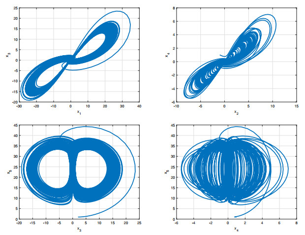
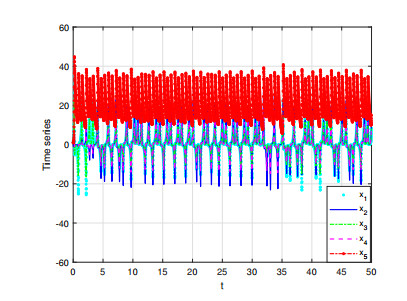
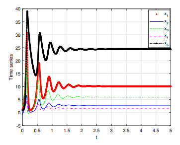
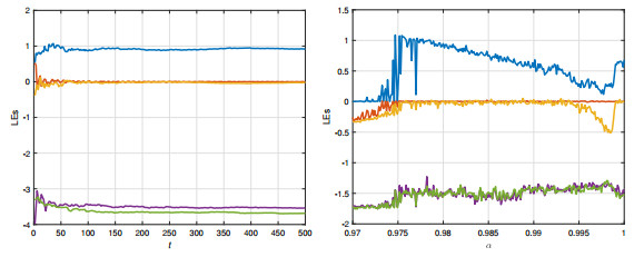
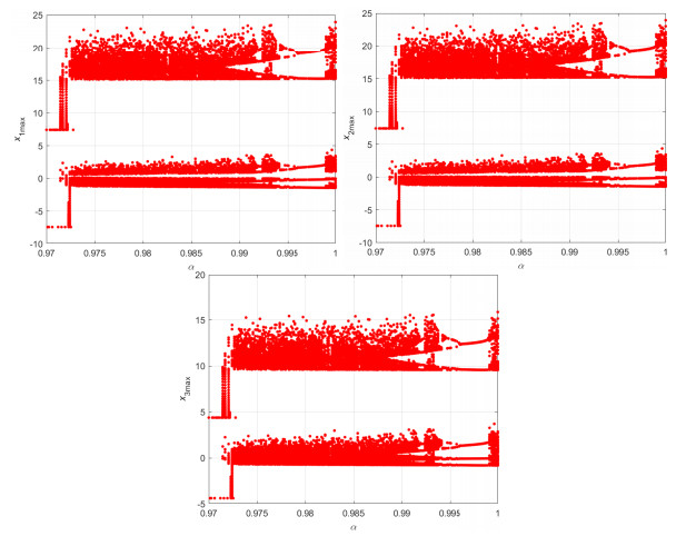
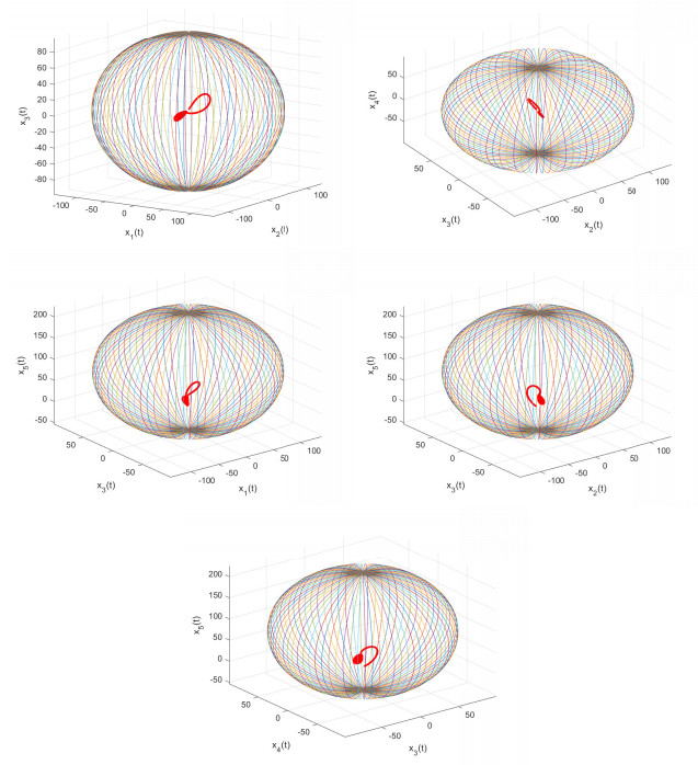
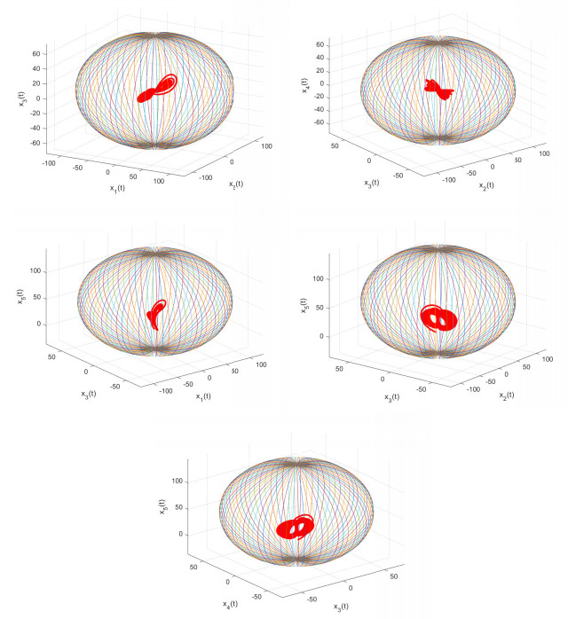
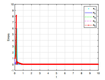
This paper presents a chaotic complex system with a fractional-order derivative. The dynamical behaviors of the proposed system such as phase portraits, bifurcation diagrams, and the Lyapunov exponents are investigated. The main contribution of this effort is an implementation of Mittag-Leffler boundedness. The global attractive sets (GASs) and positive invariant sets (PISs) for the fractional chaotic complex system are derived based on the Lyapunov stability theory and the Mittag-Leffler function. Furthermore, an effective control strategy is also designed to achieve the global synchronization of two fractional chaotic systems. The corresponding boundedness is numerically verified to show the effectiveness of the theoretical analysis.
Citation: Minghung Lin, Yiyou Hou, Maryam A. Al-Towailb, Hassan Saberi-Nik. The global attractive sets and synchronization of a fractional-order complex dynamical system[J]. AIMS Mathematics, 2023, 8(2): 3523-3541. doi: 10.3934/math.2023179
This paper presents a chaotic complex system with a fractional-order derivative. The dynamical behaviors of the proposed system such as phase portraits, bifurcation diagrams, and the Lyapunov exponents are investigated. The main contribution of this effort is an implementation of Mittag-Leffler boundedness. The global attractive sets (GASs) and positive invariant sets (PISs) for the fractional chaotic complex system are derived based on the Lyapunov stability theory and the Mittag-Leffler function. Furthermore, an effective control strategy is also designed to achieve the global synchronization of two fractional chaotic systems. The corresponding boundedness is numerically verified to show the effectiveness of the theoretical analysis.

| [1] |
A. Dlamini, E. Doungmo Goufo, M. Khumalo, On the Caputo-Fabrizio fractal fractional representation for the Lorenz chaotic system, AIMS Mathematics, 6 (2021), 12395–12421. http://dx.doi.org/10.3934/math.2021717 doi: 10.3934/math.2021717

|
| [2] |
S. David, J. Machado, D. Quintino, J. Balthazar, Partial chaos suppression in a fractional-order macroeconomic model, Math. Comput. Simulat., 122 (2016), 55–68. http://dx.doi.org/10.1016/j.matcom.2015.11.004 doi: 10.1016/j.matcom.2015.11.004
|
| [3] |
E. Bonyah, Chaos in a 5-D hyperchaotic system with four wings in the light of non-local and non-singular fractional derivatives, Chaos Soliton. Fract., 116 (2018), 316–331. http://dx.doi.org/10.1016/j.chaos.2018.09.034 doi: 10.1016/j.chaos.2018.09.034
|
| [4] |
E. Mahmoud, P. Trikha, L. Jahanzaib, O. Almaghrabi, Dynamical analysis and chaos control of the fractional chaotic ecological model, Chaos Soliton. Fract., 141 (2020), 110348. http://dx.doi.org/10.1016/j.chaos.2020.110348 doi: 10.1016/j.chaos.2020.110348
|
| [5] |
V. Pham, S. Kingni, C. Volos, S. Jafari, T. Kapitaniak, A simple three-dimensional fractional-order chaotic system without equilibrium: dynamics, circuitry implementation, chaos control and synchronization, AEU-Int. J. Electron. C., 78 (2017), 220–227. http://dx.doi.org/10.1016/j.aeue.2017.04.012 doi: 10.1016/j.aeue.2017.04.012
|
| [6] |
Y. He, J. Peng, S. Zheng, Fractional-order financial system and fixed-time synchronization, Fractal Fract., 6 (2022), 507. http://dx.doi.org/10.3390/fractalfract6090507 doi: 10.3390/fractalfract6090507
|
| [7] |
Y. Xu, Y. Li, D. Liu, Response of fractional oscillators with viscoelastic term under random excitation, J. Comput. Nonlinear Dyn., 9 (2014), 031015. http://dx.doi.org/10.1115/1.4026068 doi: 10.1115/1.4026068
|
| [8] | Z. Jiao, Y. Chen, I. Podlubny, Distributed-order dynamic systems, London: Springer, 2012. http://dx.doi.org/10.1007/978-1-4471-2852-6 |
| [9] |
B. Xu, D. Chen, H. Zhang, F. Wang, Modeling and stability analysis of a fractional-order Francis hydro-turbine governing system, Chaos Soliton. Fract., 75 (2015), 50–61. http://dx.doi.org/10.1016/j.chaos.2015.01.025 doi: 10.1016/j.chaos.2015.01.025
|
| [10] |
K. Rajagopal, A. Bayani, S. Jafari, A. Karthikeyan, I. Hussain, Chaotic dynamics of a fractional-order glucoseinsulin regulatory system, Front. Inform. Technol. Electron. Eng., 21 (2020), 1108–1118. http://dx.doi.org/10.1631/FITEE.1900104 doi: 10.1631/FITEE.1900104
|
| [11] |
M. Farmani Ardehaei, M. Farahi, S. Effati, Finite time synchronization of fractional chaotic systems with several slaves in an optimal manner, Phys. Scr., 95 (2020), 035219. http://dx.doi.org/10.1088/1402-4896/ab474d doi: 10.1088/1402-4896/ab474d
|
| [12] |
H. An, D. Feng, L. Sun, H. Zhu, The fractional-order unified chaotic system: A general cascade synchronization method and application, AIMS Mathematics, 5 (2020), 4345–4356. http://dx.doi.org/10.3934/math.2020277 doi: 10.3934/math.2020277
|
| [13] |
W. Shammakh, E. Mahmoud, B. Kashkari, Complex modified projective phase synchronization of nonlinear chaotic frameworks with complex variables, Alex. Eng. J., 59 (2020), 1265–1273. http://dx.doi.org/10.1016/j.aej.2020.02.019 doi: 10.1016/j.aej.2020.02.019
|
| [14] |
M. Aghababa, Finite-time chaos control and synchronization of fractional-order nonautonomous chaotic (hyperchaotic) systems using fractional nonsingular terminal sliding mode technique, Nonlinear Dyn., 69 (2012), 247–261. http://dx.doi.org/10.1007/s11071-011-0261-6 doi: 10.1007/s11071-011-0261-6
|
| [15] |
C. Li, J. Zhang, Synchronisation of a fractional-order chaotic system using finite-time input-to-state stability, Int. J. Syst. Sci., 47 (2016), 2440–2448. http://dx.doi.org/10.1080/00207721.2014.998741 doi: 10.1080/00207721.2014.998741
|
| [16] |
R. Behinfaraz, M. Badamchizadeh, Optimal synchronization of two different in-commensurate fractional-order chaotic systems with fractional cost function, Complexity, 21 (2016), 401–416. http://dx.doi.org/10.1002/cplx.21754 doi: 10.1002/cplx.21754
|
| [17] |
M. Tavazoei, M. Haeri, Synchronization of chaotic fractional-order systems via active sliding mode controller, Physica A, 387 (2008), 57–70. http://dx.doi.org/10.1016/j.physa.2007.08.039 doi: 10.1016/j.physa.2007.08.039
|
| [18] |
X. Zhang, Z. Li, D. Chang, Dynamics, circuit simulation and synchronization of a new three-dimensional fractional-order chaotic system, AEU-Int. J. Electron. C., 82 (2017), 435–445. http://dx.doi.org/10.1016/j.aeue.2017.10.020 doi: 10.1016/j.aeue.2017.10.020
|
| [19] |
S. Wang, S. Zheng, L. Cui, Finite-time projective synchronization and parameter identification of fractional-order complex networks with unknown external disturbances, Fractal Fract., 6 (2022), 298. http://dx.doi.org/10.3390/fractalfract6060298 doi: 10.3390/fractalfract6060298
|
| [20] | X. Liao, On the global basin of attraction and positively invariant set for the Lorenz chaotic system and its application in chaos control and synchronization, Sci. China Ser. E, 34 (2004), 1404–1419. |
| [21] |
P. Wang, Y. Zhang, S. Tan, L. Wan, Explicit ultimate bound sets of a new hyper-chaotic system and its application in estimating the Hausdorff dimension, Nonlinear Dyn., 74 (2013), 133–142. http://dx.doi.org/10.1007/s11071-013-0953-1 doi: 10.1007/s11071-013-0953-1
|
| [22] |
J. Jian, Z. Zhao, New estimations for ultimate boundary and synchronization control for a disk dynamo system, Nonlinear Anal.-Hybri., 9 (2013), 56–66. http://dx.doi.org/10.1016/j.nahs.2012.12.002 doi: 10.1016/j.nahs.2012.12.002
|
| [23] |
J. Wang, Q. Zhang, Z. Chen, H. Li, Ultimate bound of a 3D chaotic system and its application in chaos synchronization, Abstr. Appl. Anal., 2014 (2014), 781594. http://dx.doi.org/10.1155/2014/781594 doi: 10.1155/2014/781594
|
| [24] |
X. Zhang, Dynamics of a class of nonautonomous Lorenz-type systems, Int. J. Bifurcat. Chaos, 26 (2016), 1650208. http://dx.doi.org/10.1142/S0218127416502084 doi: 10.1142/S0218127416502084
|
| [25] |
F. Chien, A. Roy Chowdhury, H. Saberi Nik, Competitive modes and estimation of ultimate bound sets for a chaotic dynamical financial system, Nonlinear Dyn., 106 (2021), 3601–3614. http://dx.doi.org/10.1007/s11071-021-06945-8 doi: 10.1007/s11071-021-06945-8
|
| [26] |
F. Chien, M. Inc, H. Yosefzade, H. Saberi Nik, Predicting the chaos and solution bounds in a complex dynamical system, Chaos Soliton. Fract., 153 (2021), 111474. http://dx.doi.org/10.1016/j.chaos.2021.111474 doi: 10.1016/j.chaos.2021.111474
|
| [27] |
G. Leonov, A. Bunin, N. Koksch, Attraktorlokalisierung des Lorenz-Systems, ZAMM, 67 (1987), 649–656. http://dx.doi.org/10.1002/zamm.19870671215 doi: 10.1002/zamm.19870671215
|
| [28] | G. Leonov, Lyapunov dimension formulas for Henon and Lorenz attractors, St Petersb. Math. J., 13 (2001), 1–12. |
| [29] |
G. Leonov, Lyapunov functions in the attractors dimension theory, J. Appl. Math. Mech., 76 (2012), 129–141. http://dx.doi.org/10.1016/j.jappmathmech.2012.05.002 doi: 10.1016/j.jappmathmech.2012.05.002
|
| [30] |
P. Swinnerton-Dyer, Bounds for trajectories of the Lorenz equations:an illustration of how to choose Liapunov functions, Phys. Lett. A, 281 (2001), 161–167. http://dx.doi.org/10.1016/S0375-9601(01)00109-8 doi: 10.1016/S0375-9601(01)00109-8
|
| [31] |
F. Zhang, X. Liao, Y. Chen, C. Mu, G. Zhang, On the dynamics of the chaotic general Lorenz system, Int. J. Bifurcat. Chaos., 27 (2017), 1750075. http://dx.doi.org/10.1142/S0218127417500754 doi: 10.1142/S0218127417500754
|
| [32] |
H. Saberi Nik, S. Effati, J. Saberi-Nadjafi, New ultimate bound sets and exponential finite-time synchronization for the complex Lorenz system, J. Complexity, 31 (2015), 715–730. http://dx.doi.org/10.1016/j.jco.2015.03.001 doi: 10.1016/j.jco.2015.03.001
|
| [33] |
W. Gao, L. Yan, M. Saeedi, H. Saberi Nik, Ultimate bound estimation set and chaos synchronization for a financial risk system, Math. Comput. Simulat., 154 (2018), 19–33. http://dx.doi.org/10.1016/j.matcom.2018.06.006 doi: 10.1016/j.matcom.2018.06.006
|
| [34] | D. Kumar, S. Kumar, Ultimate numerical bound estimation of chaotic dynamical finance model, In: Modern mathematical methods and high performance computing in science and technology, Singapore: Springer, 2016, 71–81. http://dx.doi.org/10.1007/978-981-10-1454-3_6 |
| [35] |
J. Jian, K. Wu, B. Wang, Global Mittag-Leffler boundedness and synchronization for fractional-order chaotic systems, Physica A, 540 (2020), 123166. http://dx.doi.org/10.1016/j.physa.2019.123166 doi: 10.1016/j.physa.2019.123166
|
| [36] |
Q. Peng, J. Jian, Estimating the ultimate bounds and synchronization of fractional-order plasma chaotic systems, Chaos Soliton. Fract., 150 (2021), 111072. http://dx.doi.org/10.1016/j.chaos.2021.111072 doi: 10.1016/j.chaos.2021.111072
|
| [37] |
P. Wan, J. Jian, Global Mittag-Leffler boundedness for fractional-order complex-valued Cohen-Grossberg neural networks, Neural Process. Lett., 49 (2019), 121–139. http://dx.doi.org/10.1007/s11063-018-9790-z doi: 10.1007/s11063-018-9790-z
|
| [38] |
J. Jian, K. Wu, B. Wang, Global Mittag-Leffler boundedness of fractional-order fuzzy quaternion-valued neural networks with linear threshold neurons, IEEE Trans. Fuzzy Syst., 29 (2021), 3154–3164. http://dx.doi.org/10.1109/TFUZZ.2020.3014659 doi: 10.1109/TFUZZ.2020.3014659
|
| [39] |
G. Mahmoud, M. Al-Kashif, A. Farghaly, Chaotic and hyperchaotic attractors of a complex nonlinear system, J. Phys. A: Math. Theor., 41 (2008), 055104. http://dx.doi.org/10.1088/1751-8113/41/5/055104 doi: 10.1088/1751-8113/41/5/055104
|
| [40] |
Q. Wei, X. Wang, X. Hu, Adaptive hybrid complex projective synchronization of chaotic complex system, Trans. Inst. Meas. Control, 36 (2014), 1093–1097. http://dx.doi.org/10.1177/0142331214534722 doi: 10.1177/0142331214534722
|


Figures(11)

Minghung Lin, Yiyou Hou, Maryam A. Al-Towailb, Hassan Saberi-Nik. The global attractive sets and synchronization of a fractional-order complex dynamical system[J]. AIMS Mathematics, 2023, 8(2): 3523-3541. doi: 10.3934/math.2023179


 DownLoad: