Diseases of respiratory tract in young children are often accompanied by the development of bronchial obstruction syndrome. Recurrent episodes of bronchial obstruction are a common problem in young children with respiratory disorders in neonatal period. The aim of our work was to test secondary prophylactic measures concerning development and progression of recurrent bronchial obstructive syndrome in young children, who had suffered respiratory disorders in neonatal period. Prophylactic complex included basic therapy (inhalation of glucocorticosteroids—fluticasone propionate or budesonide), administration of immunomodulating drug Ribomunyl and conducting of prophylactic vaccination in specialized inpatient department after prior preparation whith antihistamines.
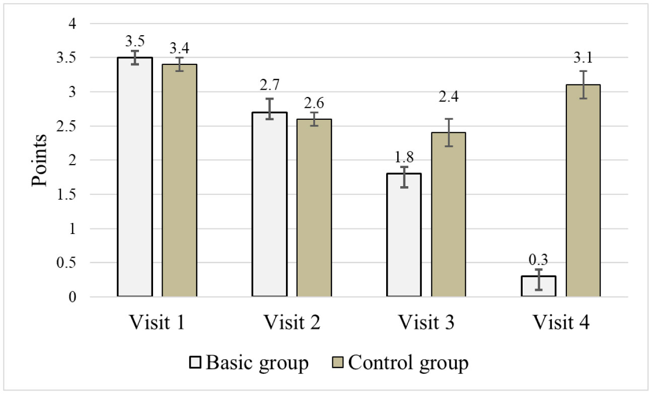
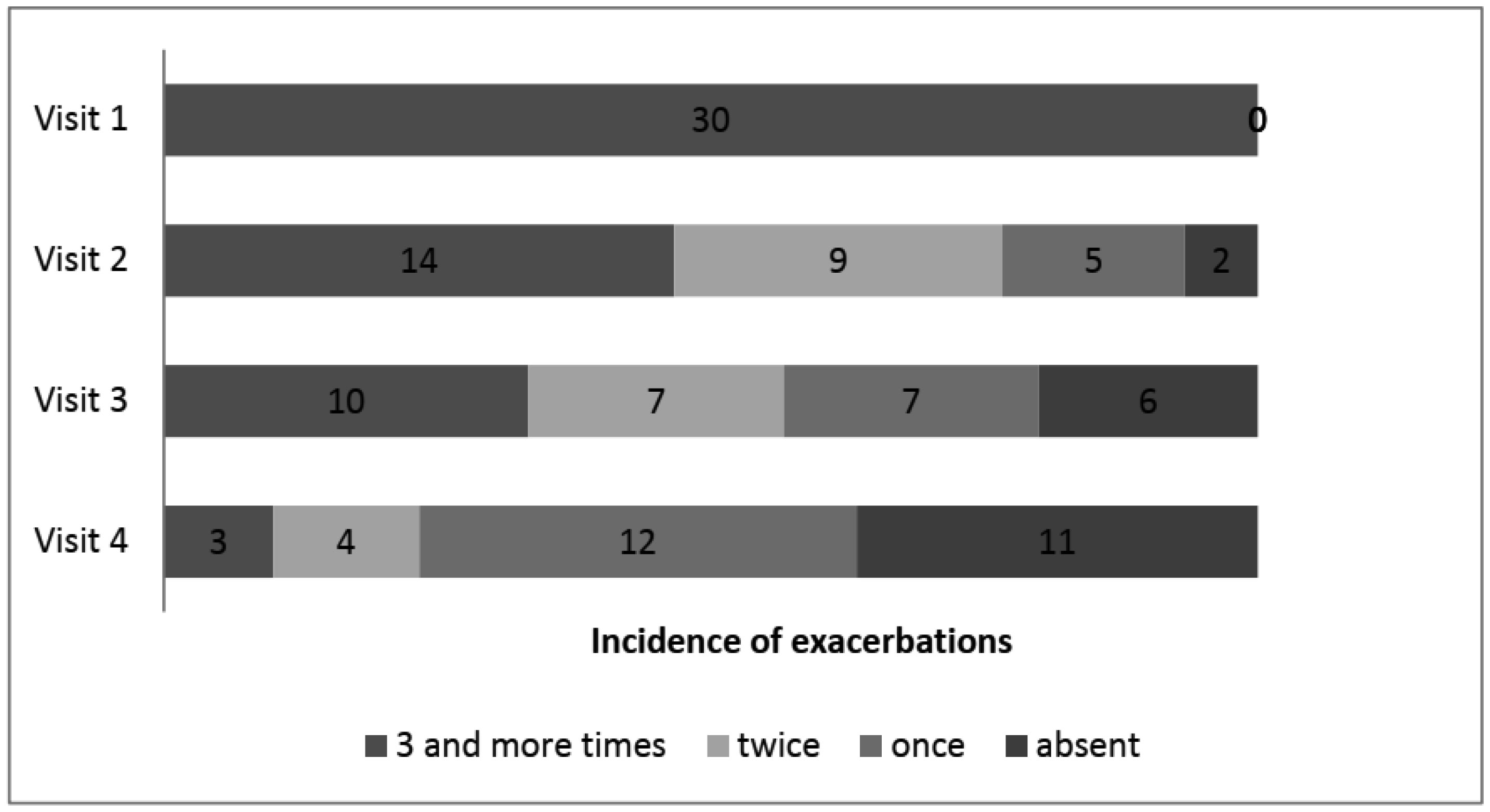
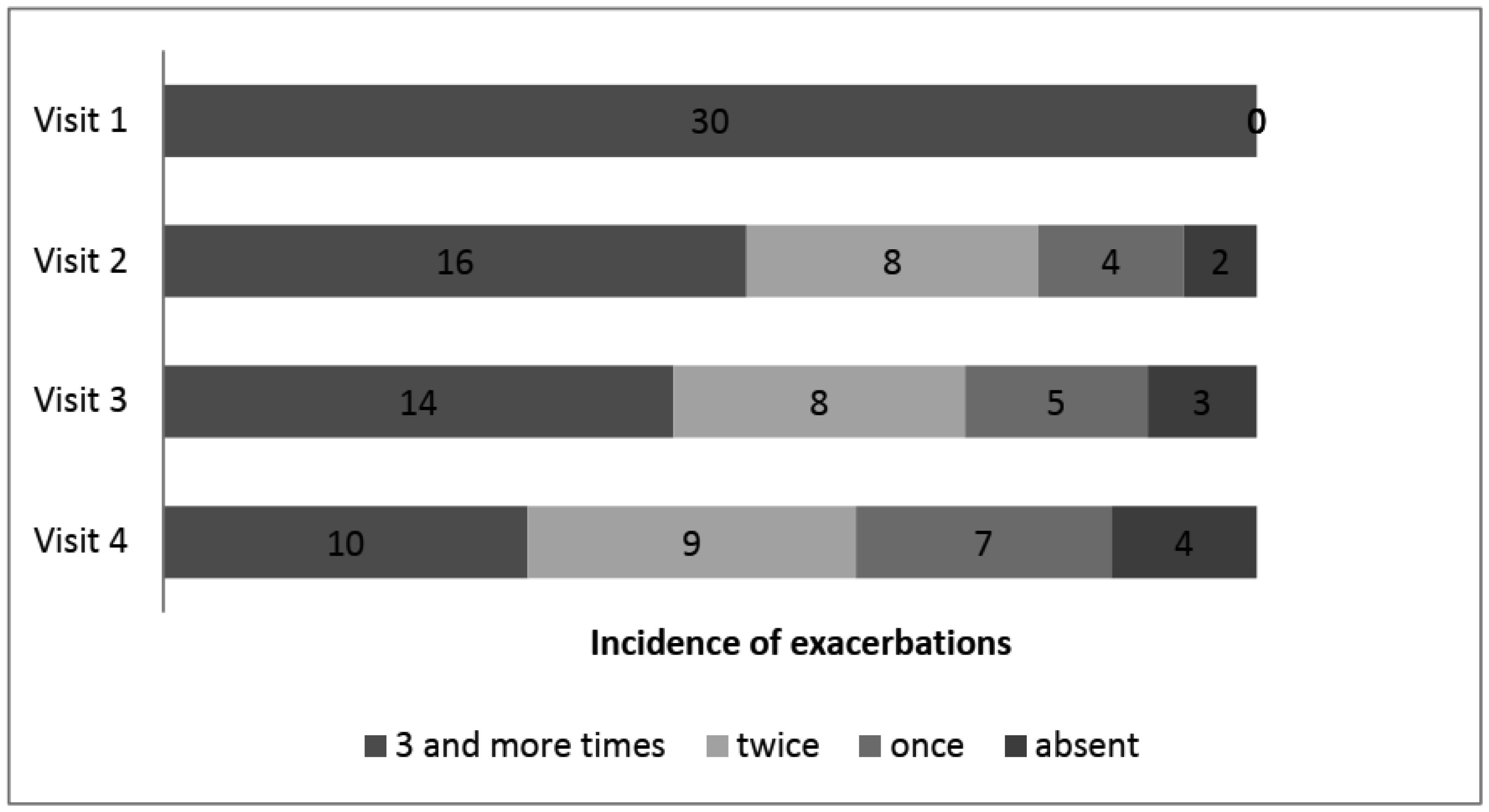
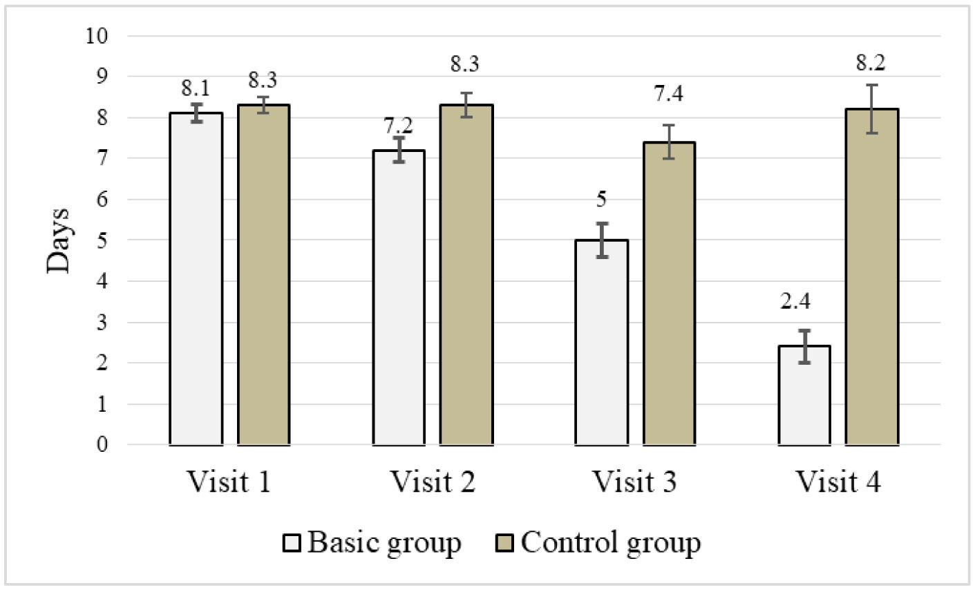
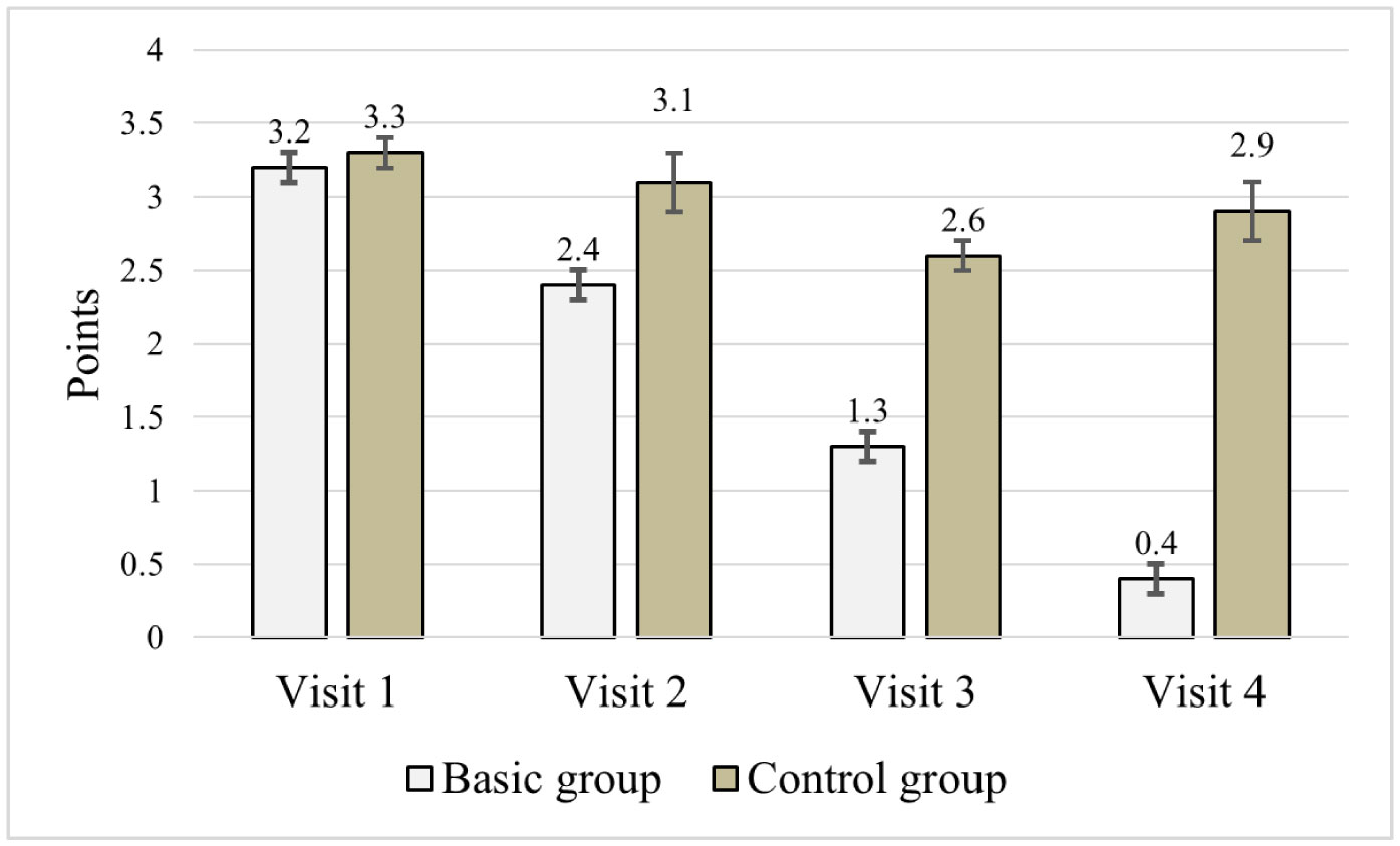
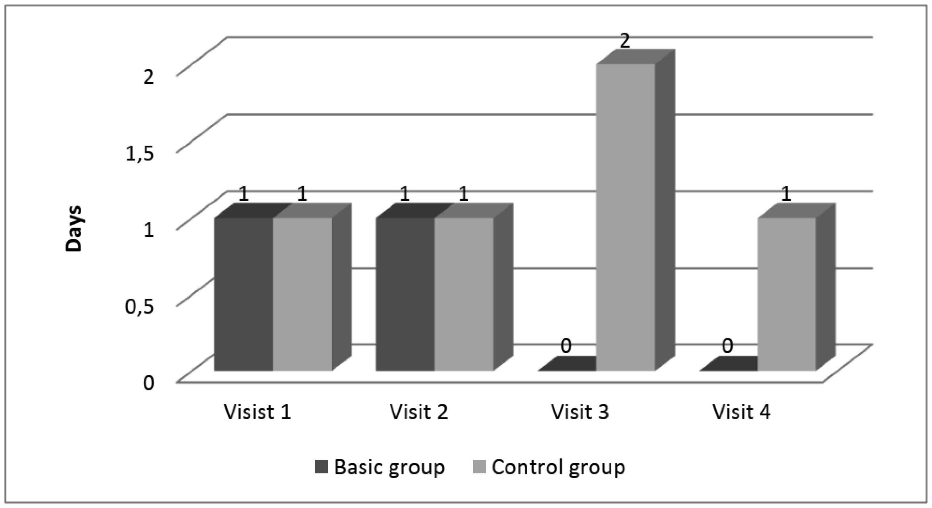
The feature of disease course was assessed based on the need of using drugs with symptomatic action, frequency of exacerbations, their mean duration and severity in 60 children, who had breathing disorders in neonatal period. Children were randomly divided into two groups. The study of efficacy of secondary prophylactic measures was conducted in 30 children (basic group) and in other 30 patients secondary prophylactic complex was not used (control group).
Algorithm of secondary prophylactic complex included basic therapy involving inhalation glucocorticosteroids, administration of immunomodulatory drug Ribomunyl as recommended and conduction of planned prophylactic inoculations with the use of antihistamines.
In children, who were administered secondary prophylactic complex was a positive dynamics in clinical picture and laboratory data.
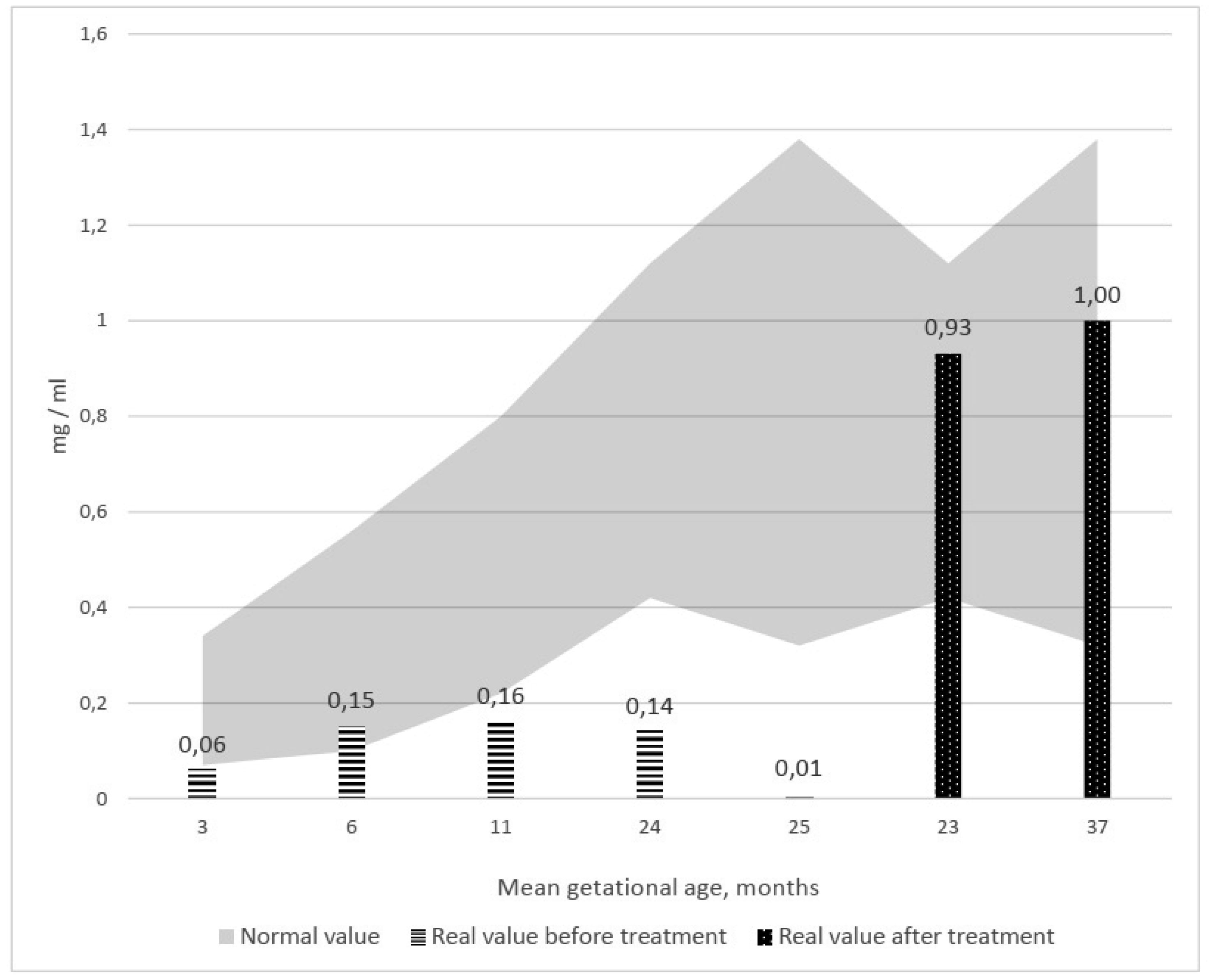
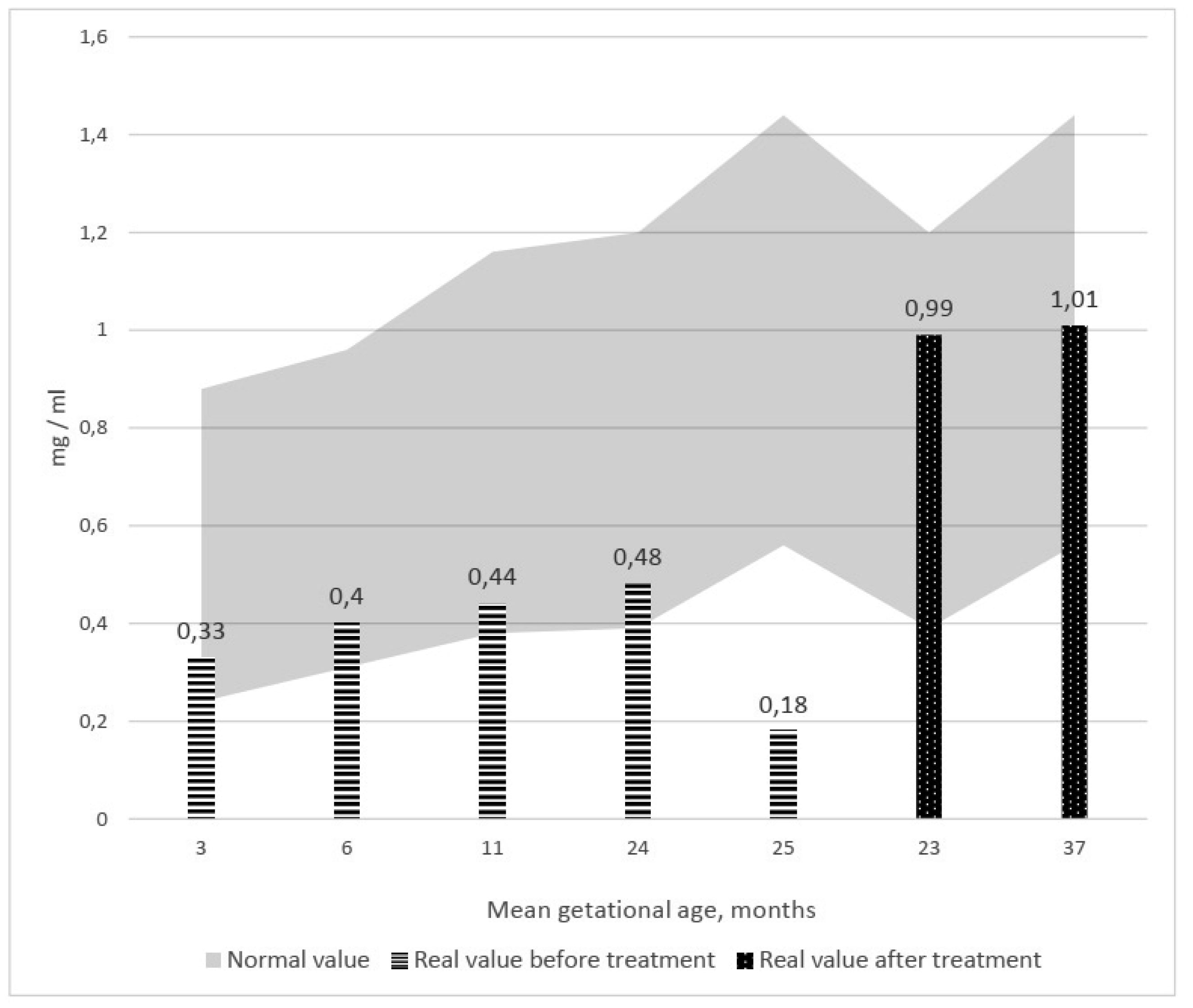
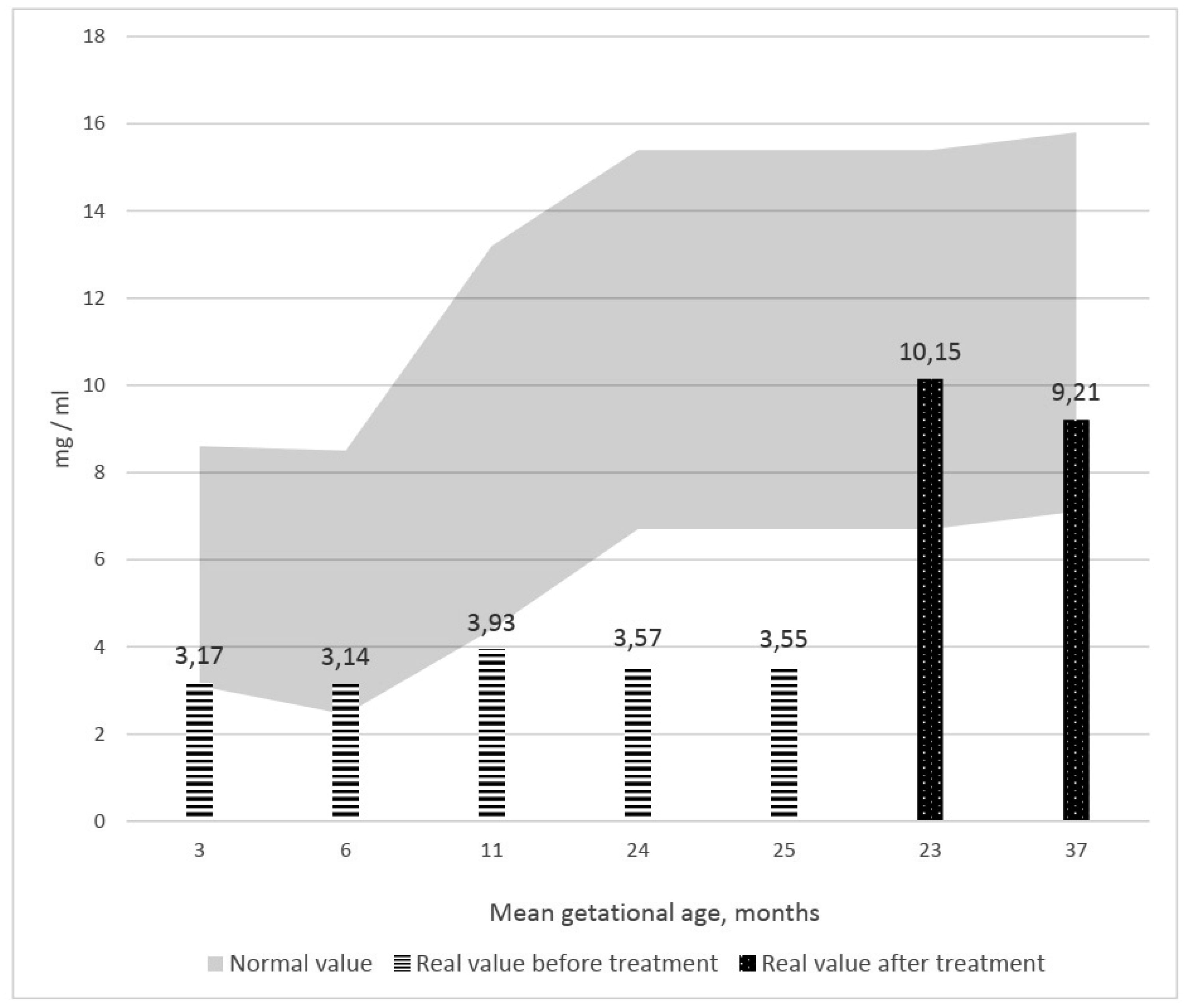
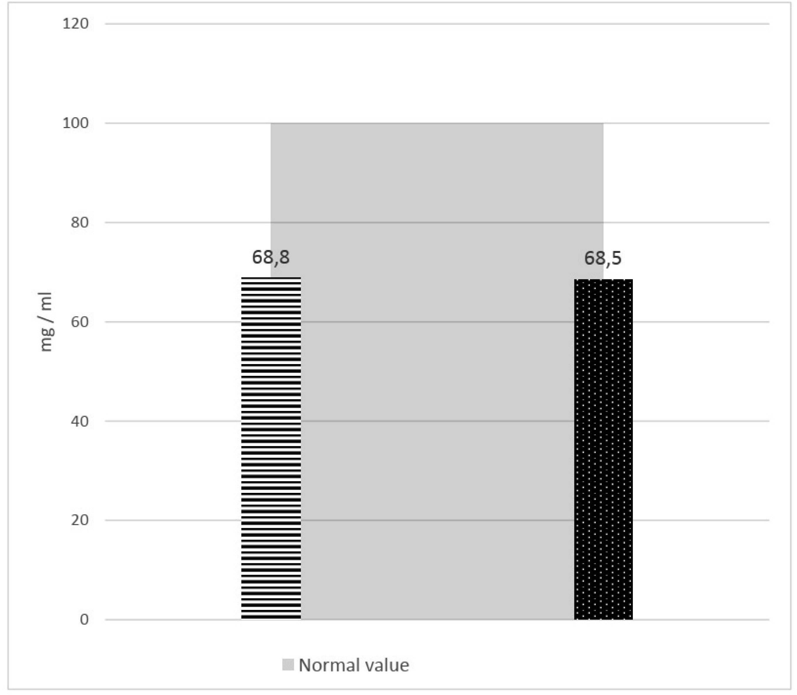
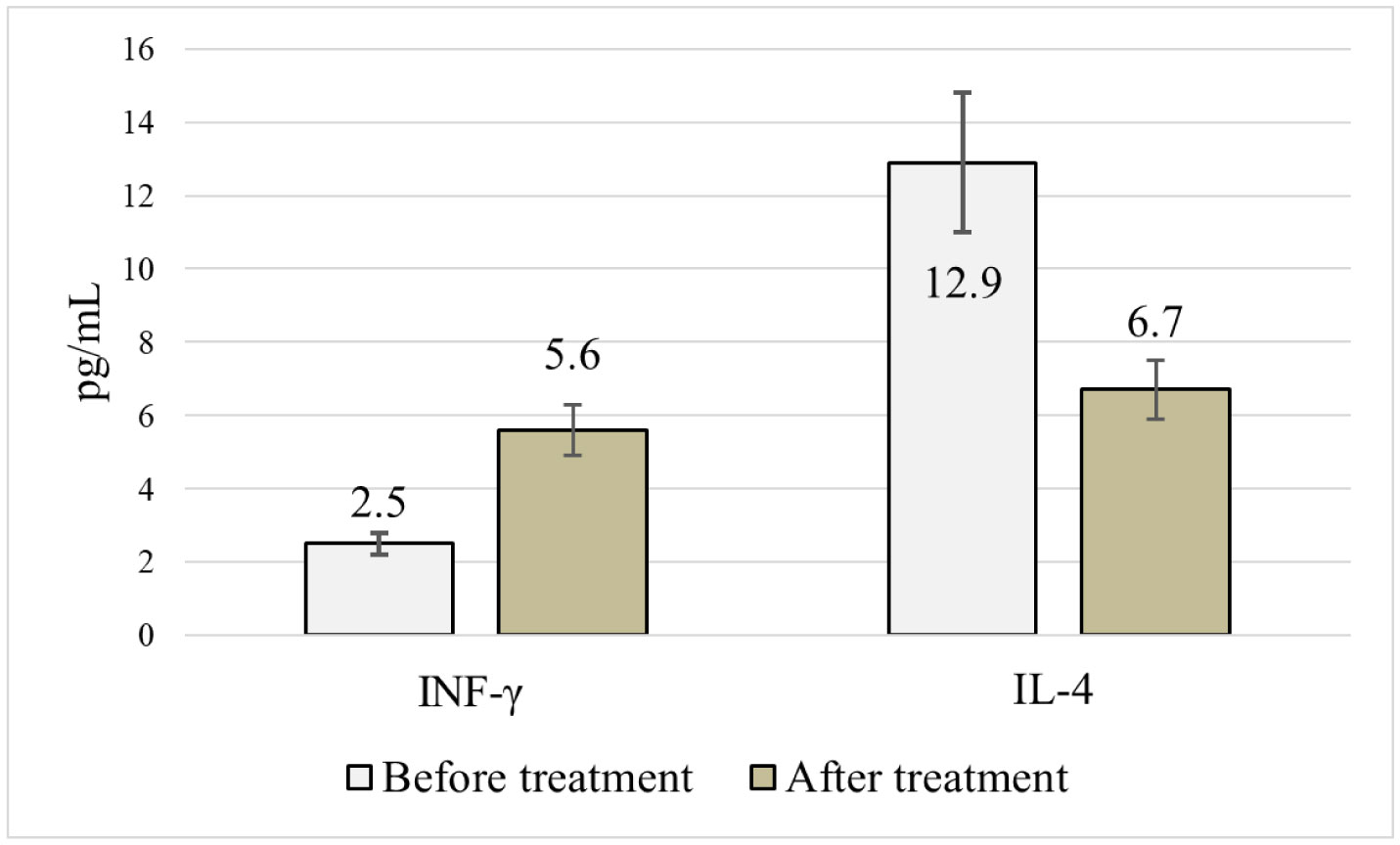
Administration of secondary prophylactic complex enabled, to a certain extent, to prevent progression of bronchial obstructive syndrome and achieve a reliable increase in γ-INF, IgA, IgM, IgG levels and decrease in IL-4 (р < 0.01).
Citation: Matsyura Oksana, Besh Lesya, Zubchenko Svitlana, Gutor Taras, Lukyanenko Natalia, Slivinska-Kurchak Khrystyna, Borysiuk Olena. Assessment of efficacy of secondary prophylactic complex of bronchial obstruction syndrome in young children with respiratory disorders in neonatal period: analysis of symptoms and serological markers[J]. AIMS Allergy and Immunology, 2022, 6(2): 25-41. doi: 10.3934/Allergy.2022005
Diseases of respiratory tract in young children are often accompanied by the development of bronchial obstruction syndrome. Recurrent episodes of bronchial obstruction are a common problem in young children with respiratory disorders in neonatal period. The aim of our work was to test secondary prophylactic measures concerning development and progression of recurrent bronchial obstructive syndrome in young children, who had suffered respiratory disorders in neonatal period. Prophylactic complex included basic therapy (inhalation of glucocorticosteroids—fluticasone propionate or budesonide), administration of immunomodulating drug Ribomunyl and conducting of prophylactic vaccination in specialized inpatient department after prior preparation whith antihistamines.
The feature of disease course was assessed based on the need of using drugs with symptomatic action, frequency of exacerbations, their mean duration and severity in 60 children, who had breathing disorders in neonatal period. Children were randomly divided into two groups. The study of efficacy of secondary prophylactic measures was conducted in 30 children (basic group) and in other 30 patients secondary prophylactic complex was not used (control group).
Algorithm of secondary prophylactic complex included basic therapy involving inhalation glucocorticosteroids, administration of immunomodulatory drug Ribomunyl as recommended and conduction of planned prophylactic inoculations with the use of antihistamines.
In children, who were administered secondary prophylactic complex was a positive dynamics in clinical picture and laboratory data.
Administration of secondary prophylactic complex enabled, to a certain extent, to prevent progression of bronchial obstructive syndrome and achieve a reliable increase in γ-INF, IgA, IgM, IgG levels and decrease in IL-4 (р < 0.01).
obstructive bronchitis
bronchial asthma
immunoglobulin
T-helpers I
T-helpers IІ
γ-interferon
interleukin
secondary prophylactic complex
tetramethylbenzidine
bronchial obstruction syndrome
corticosteroids
acute respiratory viral infections

| [1] | Rodych O, Korzhynskyy Y, Gutor T (2015) Standards of birth weight according to gestational age in the northwestern regions of Ukraine. Acta Medica Bulg 42: 34-42. https://doi.org/10.1515/amb-2015-0005 |
| [2] | Duda L, Okhotnikova O, Sharikadze O, et al. (2019) Comparative analysis of prevalence of the most common alergy diseases in children of the Kyiv region (Ukraine). Georgian Med News 6: 53-58. |
| [3] | Isayama T, Chai-Adisaksopha C, McDonald SD (2015) Noninvasive ventilation with vs without early surfactant to prevent chronic lung disease in preterm infants: a systematic review and meta-analysis. JAMA Pediatr 169: 731-739. https://doi.org/10.1001/jamapediatrics.2015.0510 |
| [4] | Clyman RI, Couto J, Murphy GM (2012) Patent ductus arteriosus: are current neonatal treatment options better or worse than no treatment at all?. Semin Perinatol 36: 123-129. https://doi.org/10.1053/j.semperi.2011.09.022 |
| [5] | Papile LA, Baley JE, Benitz W, et al. (2014) Respiratory support in preterm infants at birth. Pediatrics 133: 171-174. https://doi.org/10.1542/peds.2013-3442 |
| [6] | Bell EF, Acarregui MJ (2008) Restricted versus liberal water intake for preventing morbidity and mortality in preterm infants. Cochrane Database Syst Rev 2008: CD000503. https://doi.org/10.1002/14651858.CD000503.pub2 |
| [7] | Rabi Y, Lodha A, Soraisham A, et al. (2015) Outcomes of preterm infants following the introduction of room air resuscitation. Resuscitation 96: 252-259. https://doi.org/10.1016/j.resuscitation.2015.08.012 |
| [8] | Force ADT, Ranieri VM, Rubenfeld G, et al. (2012) Acute respiratory distress syndrome. JAMA 307: 2526-2533. https://doi.org/10.1001/jama.2012.5669 |
| [9] | Bila G, Schneider M, Peshkova S, et al. (2020) Novel approach for discrimination of eosinophilic granulocytes and evaluation of their surface receptors in a multicolor fluorescent histological assessment. Ukr Biochem J 92: 99-106. https://doi.org/10.15407/ubj92.02.099 |
| [10] | Akasaki S, Matsushita K, Kato Y, et al. (2016) Murine allergic rhinitis and nasal Th2 activation are mediated via TSLP- and IL-33-signaling pathways. Int Immunol 28: 65-76. https://doi.org/10.1093/intimm/dxv055 |
| [11] | Klonowska J, Gleń J, Nowicki RJ, et al. (2018) New cytokines in the pathogenesis of atopic dermatitis—new therapeutic targets. Int J Mol Sci 19: 3086. https://doi.org/10.3390/ijms19103086 |
| [12] | Di Cara G, Panfili E, Marseglia GL, et al. (2017) Association between pollen exposure and nasal cytokines in grass pollen-allergic children. J Invest Allerg Clin 27: 261-263. https://doi.org/10.18176/jiaci.0161 |
| [13] | Krzystek-Korpacka M, Diakowska D, Neubauer K, et al. (2013) Circulating midkine in malignant and non-malignant colorectal diseases. Cytokine 64: 158-164. https://doi.org/10.1016/j.cyto.2013.07.008 |
| [14] | Nair V, Loganathan P, Soraisham AS (2014) Azithromycin and other macrolides for prevention of bronchopulmonary dysplasia: a systematic review and meta-analysis. Neonatology 106: 337-347. https://doi.org/10.1159/000363493 |
| [15] | Sharikadze O, Zubchenko S, Maruniak S, et al. (2018) Investigation of protective effects of synbiotics on allergopathy formation. Georgian Med News 7–8: 90-94. |
| [16] | Molofsky AB, Van Gool F, Liang HE, et al. (2015) Interleukin-33 and interferon-γ counter-regulate group 2 innate lymphoid cell activation during immune perturbation. Immunity 43: 161-174. https://doi.org/10.1016/j.immuni.2015.05.019 |
Figures(11) / Tables(1)

Matsyura Oksana, Besh Lesya, Zubchenko Svitlana, Gutor Taras, Lukyanenko Natalia, Slivinska-Kurchak Khrystyna, Borysiuk Olena. Assessment of efficacy of secondary prophylactic complex of bronchial obstruction syndrome in young children with respiratory disorders in neonatal period: analysis of symptoms and serological markers[J]. AIMS Allergy and Immunology, 2022, 6(2): 25-41. doi: 10.3934/Allergy.2022005


 DownLoad: