Healthcare workers have experienced considerable stress and burnout during the COVID-19 pandemic. Among these healthcare workers are medical laboratory professionals and rehabilitation specialists, specifically, occupational therapists, and physical therapists, who all perform critical services for the functioning of a healthcare system.
This rapid review examined the impact of the pandemic on the mental health of medical laboratory professionals (MLPs), occupational therapists (OTs) and physical therapists (PTs) and identified gaps in the research necessary to understand the impact of the pandemic on these healthcare workers.
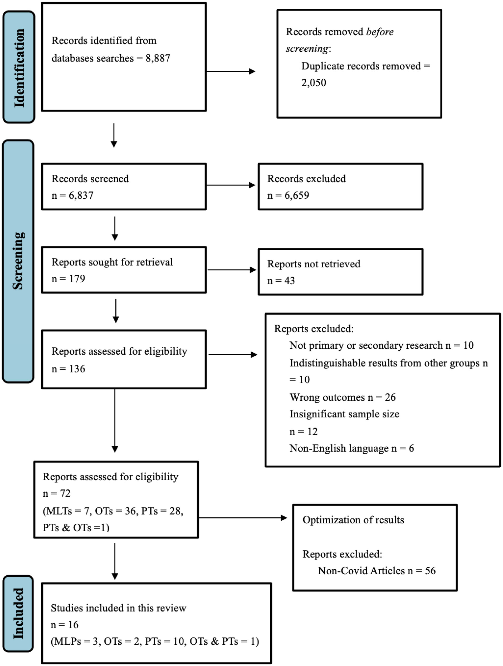
We systematically searched “mental health” among MLPs, OTs and PTs using three databases (PsycINFO, MEDLINE, and CINAHL).
Our search yielded 8887 articles, 16 of which met our criteria. Our results revealed poor mental health among all occupational groups, including burnout, depression, and anxiety. Notably, MLPs reported feeling forgotten and unappreciated compared to other healthcare groups. In general, there is a dearth of literature on the mental health of these occupational groups before and during the pandemic; therefore, unique stressors are not yet uncovered.
Our results highlight poor mental health outcomes for these occupational groups despite the dearth of research. In addition to more research among these groups, we recommend that policymakers focus on improving workplace cultures and embed more intrinsic incentives to improve job retention and reduce staff shortage. In future emergencies, providing timely and accurate health information to healthcare workers is imperative, which could also help reduce poor mental health outcomes.
Citation: Liam Ishaky, Myuri Sivanthan, Behdin Nowrouzi-Kia, Andrew Papadopoulos, Basem Gohar. The mental health of laboratory and rehabilitation specialists during COVID-19: A rapid review[J]. AIMS Public Health, 2023, 10(1): 63-77. doi: 10.3934/publichealth.2023006
Healthcare workers have experienced considerable stress and burnout during the COVID-19 pandemic. Among these healthcare workers are medical laboratory professionals and rehabilitation specialists, specifically, occupational therapists, and physical therapists, who all perform critical services for the functioning of a healthcare system.
This rapid review examined the impact of the pandemic on the mental health of medical laboratory professionals (MLPs), occupational therapists (OTs) and physical therapists (PTs) and identified gaps in the research necessary to understand the impact of the pandemic on these healthcare workers.
We systematically searched “mental health” among MLPs, OTs and PTs using three databases (PsycINFO, MEDLINE, and CINAHL).
Our search yielded 8887 articles, 16 of which met our criteria. Our results revealed poor mental health among all occupational groups, including burnout, depression, and anxiety. Notably, MLPs reported feeling forgotten and unappreciated compared to other healthcare groups. In general, there is a dearth of literature on the mental health of these occupational groups before and during the pandemic; therefore, unique stressors are not yet uncovered.
Our results highlight poor mental health outcomes for these occupational groups despite the dearth of research. In addition to more research among these groups, we recommend that policymakers focus on improving workplace cultures and embed more intrinsic incentives to improve job retention and reduce staff shortage. In future emergencies, providing timely and accurate health information to healthcare workers is imperative, which could also help reduce poor mental health outcomes.

| [1] |
Coccia M (2021) Pandemic prevention: lessons from COVID-19. Encyclopedia 1: 433-444. https://doi.org/10.3390/encyclopedia1020036 
|
| [2] |
Hruska B, Patterson PD, Doshi AA, et al. (2023) Examining the prevalence and health impairment associated with subthreshold PTSD symptoms (PTSS) among frontline healthcare workers during the COVID-19 pandemic. J Psychiatr Res 158: 202-208. https://doi.org/10.1016/j.jpsychires.2022.12.045
|
| [3] | Bose M, Mishra T, Parida S, et al. (2022) Depression, anxiety, and stress in Health care workers due to COVID-19 pandemic in hospitals of Odisha: A cross-sectional survey. J Assoc Med Sci 56: 10-18. |
| [4] |
Duarte I, Pinho R, Teixeira A, et al. (2022) Impact of COVID-19 pandemic on the mental health of healthcare workers during the first wave in Portugal: A cross-sectional and correlational study. BMJ Open 12: e064287. https://doi.org/10.1136/bmjopen-2022-064287
|
| [5] |
Nowrouzi-Kia B, Sithamparanathan G, Nadesar N, et al. (2021) Factors associated with work performance and mental health of healthcare workers during pandemics: A systematic review and meta-analysis. J Public Health 44: 731-739. https://doi.org/10.1093/pubmed/fdab173
|
| [6] |
Dos Santos Alves Maria G, de Oliveira Serpa AL, de Medeiros Chaves Ferreira C, et al. (2023) Impacts of mental health in the sleep pattern of healthcare professionals during the COVID-19 pandemic in Brazil. J Affect Disord 323: 472-481. https://doi.org/10.1016/j.jad.2022.11.082
|
| [7] |
Alalawi M, Makhlouf M, Hassanain O, et al. (2023) Healthcare workers' mental health and perception towards vaccination during COVID-19 pandemic in a pediatric cancer hospital. Sci Rep 13: 329. https://doi.org/10.1038/s41598-022-24454-5
|
| [8] |
Gohar B, Nowrouzi-Kia B (2022) The forgotten (invisible) healthcare heroes: experiences of Canadian medical laboratory employees working during the pandemic. Front Psychiatry 13: 854507. https://doi.org/10.3389/fpsyt.2022.854507
|
| [9] |
Kim SY, Kumble S, Patel B, et al. (2020) Managing the rehabilitation wave: rehabilitation services for COVID-19 survivors. Arch Phys Med Rehabil 101: 2243-2249. https://doi.org/10.1016/j.apmr.2020.09.372
|
| [10] |
Lequerica AH, Donnell CS, Tate DG (2009) Patient engagement in rehabilitation therapy: physical and occupational therapist impressions. Disabil Rehabil 31: 753-760. https://doi.org/10.1080/09638280802309095
|
| [11] |
Rogers AT, Bai G, Lavin RA, et al. (2017) Higher hospital spending on occupational therapy is associated with lower readmission rates. Med Care Res and Rev 74: 668-686. https://doi.org/10.1177/1077558716666981
|
| [12] |
Wang TJ, Chau B, Lui M, et al. (2020) Physical medicine and rehabilitation and pulmonary rehabilitation for COVID-19. Am J Phys Med Rehabil 99: 769-774. https://doi.org/10.1097/PHM.0000000000001505
|
| [13] |
Hoel V, Zweck C von, Ledgerd R (2021) The impact of Covid-19 for occupational therapy: Findings and recommendations of a global survey. World Fed Occup Thera Bull 77: 69-76. https://doi.org/10.1080/14473828.2020.1855044
|
| [14] |
Chatzittofis A, Karanikola M, Michailidou K, et al. (2021) Impact of the COVID-19 pandemic on the mental health of healthcare workers. Int J Environ Res Public Health 18: 1435. https://doi.org/10.3390/ijerph18041435
|
| [15] | Śliwiński Z, Starczyńska M, Kotela I, et al. (2014) Burnout among physiotherapists and length of service. Int J Occup Med Environ Health 27: 224-235. https://doi.org/10.2478/s13382-014-0248-x |
| [16] |
Brown CA, Schell J, Pashniak LM (2017) Occupational therapists' experience of workplace fatigue: Issues and action. Work 57: 517-527. https://doi.org/10.3233/WOR-172576
|
| [17] |
Rodríguez-Nogueira Ó, Leirós-Rodríguez R, Pinto-Carral A, et al. (2022) The relationship between burnout and empathy in physiotherapists: A cross-sectional study. Ann Med 54: 933-940. https://doi.org/10.1080/07853890.2022.2059102
|
| [18] |
Gupta S, Paterson ML, Lysaght RM, et al. (2012) Experiences of burnout and coping strategies utilized by occupational therapists. Can J Occup Ther 79: 86-95. https://doi.org/10.2182/cjot.2012.79.2.4
|
| [19] | Government of CanadaAbout Mental Health (2022). Available from: https://www.canada.ca/en/public-health/services/about-mental-health.html. |
| [20] | Veritas Health InnovationCovidence systematic review software n.d. Available from: https://www.covidence.org. |
| [21] |
Borusiak P, Mazheika Y, Bauer S, et al. (2022) The impact of the COVID-19 pandemic on pediatric developmental services: A cross-sectional study on overall burden and mental health status. Arch Public Health 80: 113. https://doi.org/10.1186/s13690-022-00876-5
|
| [22] |
Moher D, Liberati A, Tetzlaff J, et al. (2009) Preferred reporting items for systematic reviews and meta-analyses: the PRISMA statement. BMJ 339: b2535. https://doi.org/10.1136/bmj.b2535
|
| [23] |
Nowrouzi-Kia B, Dong J, Gohar B, et al. (2022) Factors associated with burnout among medical laboratory professionals in Ontario, Canada: An exploratory study during the second wave of the COVID-19 pandemic. Int J Health Plann Manage 37: 2183-2197. https://doi.org/10.1002/hpm.3460
|
| [24] |
Matsuo T, Kobayashi D, Taki F, et al. (2020) Prevalence of Health Care Worker Burnout During the Coronavirus Disease 2019 (COVID-19) Pandemic in Japan. JAMA Netw Open 3: e2017271. https://doi.org/10.1001/jamanetworkopen.2020.17271
|
| [25] |
Ishioka T, Ito A, Miyaguchi H, et al. (2021) Psychological Impact of COVID-19 on Occupational Therapists: An Online Survey in Japan. Am J Occup Ther 75: 7504205010. https://doi.org/10.5014/ajot.2021.046813
|
| [26] |
Chan M, Lee A (2022) Perceived social support and depression among occupational therapists in Hong Kong during COVID-19 pandemic. East Asian Arch. Psychiatry 32: 17-21. https://doi.org/10.12809/eaap2205
|
| [27] |
Duarte H, Daros Vieira R, Cardozo Rocon P, et al. (2022) Factors associated with Brazilian physical therapists' perception of stress during the COVID-19 pandemic: A cross-sectional survey. Psychol Health Med 27: 42-53. https://doi.org/10.1080/13548506.2021.1875133
|
| [28] |
Jácome C, Seixas A, Serrão C, et al. (2021) Burnout in Portuguese physiotherapists during COVID-19 pandemic. Physiother Res Int 26: e1915. https://doi.org/10.1002/pri.1915
|
| [29] |
Lino JA, CG Frota LG, V Abdon AP, et al. (2022) Sleep quality and associated factors amongst Brazilian physiotherapists during the COVID-19 pandemic. Physiother Theory Pract 38: 2612-2620. https://doi.org/10.1080/09593985.2021.1965271
|
| [30] |
Szwamel K, Kaczorowska A, Lepsy E, et al. (2022) Predictors of the occupational burnout of healthcare workers in Poland during the COVID-19 pandemic: A cross-sectional study. Int J Environ Res Public Health 19: 3634. https://doi.org/10.3390/ijerph19063634
|
| [31] |
Pniak B, Leszczak J, Adamczyk M, et al. (2021) Occupational burnout among active physiotherapists working in clinical hospitals during the COVID-19 pandemic in south-eastern Poland. Work 68: 285-295. https://doi.org/10.3233/WOR-203375
|
| [32] |
Yang S, Kwak SG, Ko EJ, et al. (2020) The mental health burden of the COVID-19 pandemic on physical therapists. Int J Environ Res Public Health 17: 3723. https://doi.org/10.3390/ijerph17103723
|
| [33] |
Hassem T, Israel N, Bemath N, et al. (2022) COVID-19: Contrasting experiences of South African physiotherapists based on patient exposure. S Afr J Physiother 78: 1576. https://doi.org/10.4102/sajp.v78i1.1576
|
| [34] |
Ditwiler RE, Swisher LL, Hardwick DD (2021) Professional and ethical issues in United States acute care physical therapists treating patients with COVID-19: Stress, walls, and uncertainty. Phys Ther 101: pzab122. https://doi.org/10.1093/ptj/pzab122
|
| [35] |
Palacios-Ceña D, Fernández-de-las-Peñas C, Florencio LL, et al. (2020) Emotional experience and feelings during first COVID-19 outbreak perceived by physical therapists: A qualitative study in Madrid, Spain. Int J Environ Res Public Health 18: 127. https://doi.org/10.3390/ijerph18010127
|
| [36] |
Youssef D, Youssef J, Hassan H, et al. (2021) Prevalence and risk factors of burnout among Lebanese community pharmacists in the era of COVID-19 pandemic: Results from the first national cross-sectional survey. J Pharm Policy Pract 14: 111. https://doi.org/10.1186/s40545-021-00393-w
|
| [37] | Baldonedo-Mosteiro C, Franco-Correia S, Mosteiro-Diaz MP (2022) Psychological impact of COVID19 on community pharmacists and pharmacy technicians. Explor Res Clin Soc Pharm 5: 100118. https://doi.org/10.1016/j.rcsop.2022.100118 |
| [38] |
Gohar B, Larivière M, Lightfoot N, et al. (2020) Meta-analysis of nursing-related organizational and psychosocial predictors of sickness absence. Occup Med 70: 593-601. https://doi.org/10.1093/occmed/kqaa144
|
| [39] |
Healy S, Tyrrell M (2013) Importance of debriefing following critical incidents. Emerg Nurse 20: 32-37. https://doi.org/10.7748/en2013.03.20.10.32.s8
|
| [40] | Coccia M (2019) Intrinsic and extrinsic incentives to support motivation and performance of public organizations. J Econ Bibliography 6: 20-29. https://doi.org/http://dx.doi.org/10.1453/jeb.v6i1.1795 |
| [41] |
Nocera M, Merritt C (2017) Pediatric critical event debriefing in emergency medicine training: An opportunity for educational improvement. AEM Educ Train 1: 208-214. https://doi.org/10.1002/aet2.10031
|
| [42] |
Cameron S, Armstrong-Stassen M, Bergeron S, et al. (2004) Recruitment and retention of nurses: Challenges facing hospital and community employers. Nurs Leadersh 17: 79-92. https://doi.org/10.12927/cjnl.2004.16359
|
| [43] | Razu SR, Yasmin T, Arif TB, et al. (2021) Challenges faced by healthcare professionals during the COVID-19 pandemic: A qualitative inquiry from Bangladesh. Front Public Health 9: 1024. https://doi.org/10.3389/fpubh.2021.647315 |
| [44] |
Gohar B, Larivière M, Nowrouzi-Kia B (2020) Sickness absence in healthcare workers during the COVID-19 pandemic. Occup Med 70: 338-342. https://doi.org/10.1093/occmed/kqaa093
|
| [45] |
Gohar B, Larivière M, Lightfoot N, et al. (2020) Understanding sickness absence in nurses and personal support workers: Insights from frontline staff and key informants in Northeastern Ontario. Work 66: 755-766. https://doi.org/10.3233/WOR-203222
|
Figures(1) / Tables(3)

Liam Ishaky, Myuri Sivanthan, Behdin Nowrouzi-Kia, Andrew Papadopoulos, Basem Gohar. The mental health of laboratory and rehabilitation specialists during COVID-19: A rapid review[J]. AIMS Public Health, 2023, 10(1): 63-77. doi: 10.3934/publichealth.2023006


 DownLoad: