Bipolar disorder is a psychiatric condition that consists of recurring episodes of severe mood swings between depression and manic episodes. The diagnosis is generally based on clinical interviews and observations, but is often misdiagnosed as unipolar depression, leading to significant delays in treatment. However, the disorder's heterogeneous nature and overlap with other psychiatric conditions, such as schizophrenia, present challenges in its diagnosis and treatment. To address these challenges, this study aims to explore the gene targets of differentially expressed miRNA associated with differentially expressed genes and to find a suitable phytochemical through molecular docking studies. The altered expression level of miRNAs (either increased or decreased) and genes had been observed to play a crucial role in different psychiatric disorders, thus suggesting their potential as biomarkers. The data of patients with bipolar disorder was retrieved from the Gene expression omnibus and Sequence read archive. The differentially expressed genes and miRNAs were identified through DESeq2 post processing. The gene targets of the downregulated miRNA and the upregulated genes were compared to identify the main targets of bipolar disorder. Furthermore, the phytochemicals with neuro-protective properties were identified through a literature study. The drug likeness property of each phytochemical was evaluated on the basis of Lipinski's rule of 5, followed by a toxicity evaluation. Molecular docking studies were carried out using AutoDock to determine the best drug against bipolar disorder. Therefore, the present study targets key proteins overexpressed in patients with bipolar disorder to facilitate a multi-faceted treatment approach.
Citation: Harshita Maheshwari, Maitreyi Pathak, Prekshi Garg, Prachi Srivastava. Computational analysis reveals the therapeutic potential of Asiatic acid against the miRNA correlated differentially expressed genes of bipolar disorder[J]. AIMS Molecular Science, 2024, 11(2): 99-115. doi: 10.3934/molsci.2024007
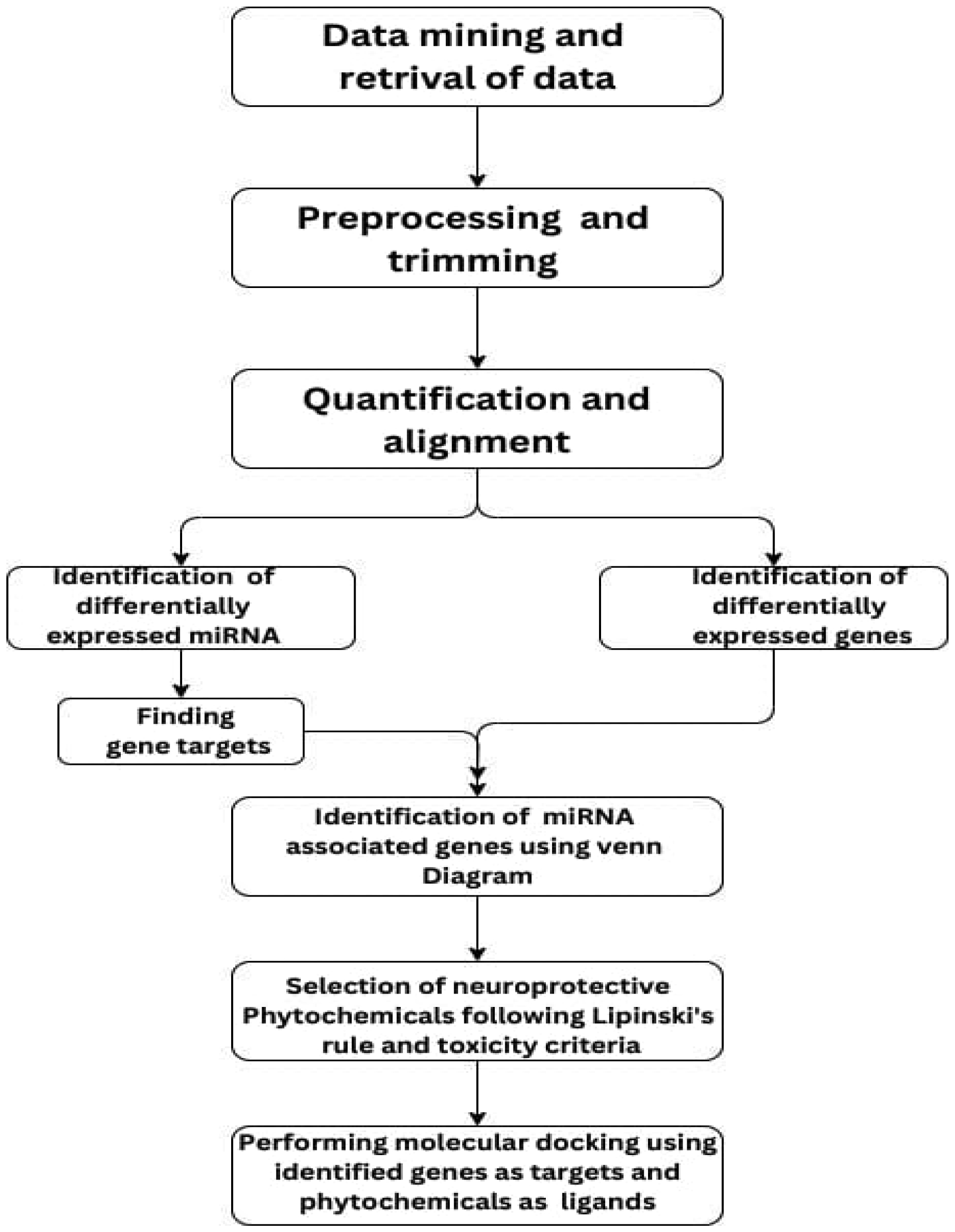
Bipolar disorder is a psychiatric condition that consists of recurring episodes of severe mood swings between depression and manic episodes. The diagnosis is generally based on clinical interviews and observations, but is often misdiagnosed as unipolar depression, leading to significant delays in treatment. However, the disorder's heterogeneous nature and overlap with other psychiatric conditions, such as schizophrenia, present challenges in its diagnosis and treatment. To address these challenges, this study aims to explore the gene targets of differentially expressed miRNA associated with differentially expressed genes and to find a suitable phytochemical through molecular docking studies. The altered expression level of miRNAs (either increased or decreased) and genes had been observed to play a crucial role in different psychiatric disorders, thus suggesting their potential as biomarkers. The data of patients with bipolar disorder was retrieved from the Gene expression omnibus and Sequence read archive. The differentially expressed genes and miRNAs were identified through DESeq2 post processing. The gene targets of the downregulated miRNA and the upregulated genes were compared to identify the main targets of bipolar disorder. Furthermore, the phytochemicals with neuro-protective properties were identified through a literature study. The drug likeness property of each phytochemical was evaluated on the basis of Lipinski's rule of 5, followed by a toxicity evaluation. Molecular docking studies were carried out using AutoDock to determine the best drug against bipolar disorder. Therefore, the present study targets key proteins overexpressed in patients with bipolar disorder to facilitate a multi-faceted treatment approach.

| [1] | Jain A, Mitra P (2023) Bipolar disorder. Available from: https://www.ncbi.nlm.nih.gov/books/NBK558998/. |
| [2] | Hilty DM, Leamon MH, Lim RF, et al. (2006) A review of bipolar disorder in adults. Psychiatry (Edgmont) 3: 43-55. |
| [3] |
Zhang N, Hu G, Myers TG, et al. (2019) Protocols for the analysis of microRNA expression, biogenesis, and function in immune cells. Curr Protoc Immunol 126: e78. https://doi.org/10.1002/cpim.78 
|
| [4] |
Filipowicz W, Bhattacharyya SN, Sonenberg N (2008) Mechanisms of post-transcriptional regulation by microRNAs: are the answers in sight?. Nat Rev Genet 9: 102-114. https://doi.org/10.1038/nrg229
|
| [5] |
Anjum A, Jaggi S, Varghese E, et al. (2016) Identification of differentially expressed genes in RNA-seq data of arabidopsis thaliana: A compound distribution approach. J Comput Biol 23: 239-247. https://doi.org/10.1089/cmb.2015.0205
|
| [6] |
Rodriguez-Esteban R, Jiang X (2017) Differential gene expression in disease: a comparison between high-throughput studies and the literature. BMC Med Genomics 10: 59. https://doi.org/10.1186/s12920-017-0293-y
|
| [7] |
Pfaffenseller B, da Silva Magalhães PV, De Bastiani MA, et al. (2016) Differential expression of transcriptional regulatory units in the prefrontal cortex of patients with bipolar disorder: potential role of early growth response gene 3. Transl Psychiatry 6: e805. https://doi.org/10.1038/tp.2016.78
|
| [8] |
Machado-Vieira R, Manji HK, Zarate CA, et al. (2009) The role of lithium in the treatment of bipolar disorder: convergent evidence for neurotrophic effects as a unifying hypothesis. Bipolar disord 11: 92-109. https://doi.org/10.1111/j.1399-5618.2009.00714.x
|
| [9] |
Qureshi NA, Al-Bedah AM (2013) Mood disorders and complementary and alternative medicine: A literature review. Neuropsychiatr Dis Treat 2013: 639-658. https://doi.org/10.2147/NDT.S43419
|
| [10] |
Clough E, Barrett T (2016) The gene expression omnibus database. Statistical genomics . New York: Humana Press 93-110. https://doi.org/10.1007/978-1-4939-3578-9_5
|
| [11] |
Leinonen R, Sugawara H, Shumway M (2011) International Nucleotide Sequence Database Collaboration. The sequence read archive. Nucleic Acids Res : D19-D21. https://doi.org/10.1093/nar/gkq1019
|
| [12] | FastQC: A quality control tool for high throughput sequence data. Available from: http://www.bioinformatics.babraham.ac.uk/projects/fastqc |
| [13] |
Jalili V, Afgan E, Gu Q, et al. (2020) The Galaxy platform for accessible, reproducible and collaborative biomedical analyses: 2020 update. Nucleic Acids Res 48: 8205-8207. https://doi.org/10.1093/nar/gkaa554
|
| [14] |
Friedländer MR, Mackowiak SD, Li N, et al. (2012) miRDeep2 accurately identifies known and hundreds of novel microRNA genes in seven animal clades. Nucleic Acids Res 40: 37-52. https://doi.org/10.1093/nar/gkr688
|
| [15] |
Kim D, Langmead B, Salzberg SL (2015) HISAT: A fast spliced aligner with low memory requirements. Nat Methods 12: 357-360. https://doi.org/10.1038/nmeth.3317
|
| [16] | Mackowiak SD (2011) Identification of novel and known miRNAs in deep-sequencing data with miRDeep2. Curr Protoc Bioinformatics . https://doi.org/10.1002/0471250953.bi1210s36 |
| [17] |
Liao Y, Smyth GK, Shi W (2014) featureCounts: An efficient general purpose program for assigning sequence reads to genomic features. Bioinformatics 30: 923-930. https://doi.org/10.1093/bioinformatics/btt656
|
| [18] |
Love MI, Huber W, Anders S (2014) Moderated estimation of fold change and dispersion for RNA-seq data with DESeq2. Genome Biol 15: 550. https://doi.org/10.1186/s13059-014-0550-8
|
| [19] |
Riffo-Campos ÁL, Riquelme I, Brebi-Mieville P (2016) Tools for sequence-based miRNA target prediction: What to choose?. Int J Mol Sci 17: 1987. https://doi.org/10.3390/ijms17121987
|
| [20] | Venny—An interactive tool for comparing lists with Venn's diagrams. Available from: https://bioinfogp.cnb.csic.es/tools/venny/index.html |
| [21] | Molinspiration cheminformatics. Available from: https://molinspiration.com/ |
| [22] |
Banerjee P, Eckert OA, Schrey AK, et al. (2018) ProTox-II: A webserver for the prediction of toxicity of chemicals. Nucleic Acids Res 46: W257-W263. https://doi.org/10.1093/nar/gky318
|
| [23] | Rizvi SMD, Shakil S, Haneef M (2013) A simple click by click protocol to perform docking: AutoDock 4.2 made easy for non-bioinformaticians. EXCLI J 12: 831-857. |
| [24] |
Pacifico R, Davis RL (2017) Transcriptome sequencing implicates dorsal striatum-specific gene network, immune response and energy metabolism pathways in bipolar disorder. Mol Psychiatry 22: 441-449. https://doi.org/10.1038/mp.2016.94
|
| [25] |
Pai S, Li P, Killinger B, et al. (2019) Differential methylation of enhancer at IGF2 is associated with abnormal dopamine synthesis in major psychosis. Nat Commun 10: 2046. https://doi.org/10.1038/s41467-019-09786-7
|
| [26] |
Hu J, Xu J, Pang L, et al. (2016) Systematically characterizing dysfunctional long intergenic non-coding RNAs in multiple brain regions of major psychosis. Oncotarget 7: 71087-71098. https://doi.org/10.18632/oncotarget.12122
|
| [27] |
Xu Z, Adilijiang A, Wang W, et al. (2019) Arecoline attenuates memory impairment and demyelination in a cuprizone-induced mouse model of schizophrenia. Neuroreport 30: 134-138. https://doi.org/10.1097/WNR.0000000000001172
|
| [28] | Suresh P, Raju AB (2013) Antidopaminergic effects of leucine and genistein on shizophrenic rat models. Neurosciences 18: 235-241. |
| [29] |
Lin JC, Lee MY, Chan MH, et al. (2016) Betaine enhances antidepressant-like, but blocks psychotomimetic effects of ketamine in mice. Psychopharmacology (Berl) 233: 3223-3235. https://doi.org/10.1007/s00213-016-4359-x
|
| [30] |
Ben-Azu B, Aderibigbe AO, Omogbiya IA, et al. (2018) Morin pretreatment attenuates schizophrenia-like behaviors in experimental animal models. Drug Res (Stuttg) 68: 159-167. https://doi.org/10.1055/s-0043-119127
|
| [31] |
Kumar G, Patnaik R (2016) Exploring neuroprotective potential of Withania somnifera phytochemicals by inhibition of GluN2B-containing NMDA receptors: An in silico study. Med Hypotheses 92: 35-43. https://doi.org/10.1016/j.mehy.2016.04.034
|
| [32] |
Chen W, Qi J, Feng F, et al. (2014) Neuroprotective effect of allicin against traumatic brain injury via Akt/endothelial nitric oxide synthase pathwaymediated anti-inflammatory and anti-oxidative activities. Neurochem Int 68: 28-37. https://doi.org/10.1016/j.neuint.2014.01.015
|
| [33] |
Zhu HT, Bian C, Yuan JC, et al. (2014) Curcumin attenuates acute inflammatory injury by inhibiting the TLR4/MyD88/NF-κB signaling pathway in experimental traumatic brain injury. J Neuroinflammation 11: 59. https://doi.org/10.1186/1742-2094-11-59
|
| [34] |
Krishnamurthy RG, Senut MC, Zemke D, et al. (2009) Asiatic acid, a pentacyclic triterpene from Centella asiatica, is neuroprotective in a mouse model of focal cerebral ischemia. J Neurosci Res 87: 2541-2550. https://doi.org/10.1002/jnr.22071
|
| [35] |
Chandrasekaran K, Mehrabian Z, Spinnewyn B, et al. (2001) Neuroprotective effects of bilobalide, a component of the Ginkgo biloba extract (EGb 761), in gerbil global brain ischemia. Brain Res 922: 282-292. https://doi.org/10.1016/S0006-8993(01)03188-2
|
| [36] |
Zhao J, Kobori N, Aronowski J, et al. (2006) Sulforaphane reduces infarct volume following focal cerebral ischemia in rodents. Neurosci Lett 393: 108-112. https://doi.org/10.1016/j.neulet.2005.09.065
|
| [37] |
Lakstygal AM, Kolesnikova TO, Khatsko SL, et al. (2019) DARK classics in chemical neuroscience: Atropine, scopolamine, and other anticholinergic deliriant hallucinogens. ACS Chem Neurosci 10: 2144-2159. https://doi.org/10.1021/acschemneuro.8b00615
|
| [38] |
Huang SS, Tsai MC, Chih CL, et al. (2001) Resveratrol reduction of infarct size in Long-Evans rats subjected to focal cerebral ischemia. Life Sci 69: 1057-1065. https://doi.org/10.1016/S0024-3205(01)01195-X
|
| [39] |
Leiderman E, Zylberman I, Zukin SR, et al. (1996) Preliminary investigation of high-dose oral glycine on serum levels and negative symptoms in schizophrenia: An open-label trial. Biol Psychiatry 39: 213-215. https://doi.org/10.1016/0006-3223(95)00585-4
|
| [40] |
Hannan MA, Rahman MA, Sohag AAM, et al. (2021) Black cumin (Nigella sativa L.): A comprehensive review on phytochemistry, health benefits, molecular pharmacology, and safety. Nutrients 13: 1784. https://doi.org/10.3390/nu13061784
|
| [41] |
Yadav M, Jindal DK, Dhingra MS, et al. (2018) Protective effect of gallic acid in experimental model of ketamine-induced psychosis: Possible behaviour, biochemical, neurochemical and cellular alterations. Inflammopharmacology 26: 413-424. https://doi.org/10.1007/s10787-017-0366-8
|
| [42] |
Mukherjee PK, Kumar V, Mal M, et al. (2007) In vitro acetylcholinesterase inhibitory activity of the essential oil from Acorus calamus and its main constituents. Planta Med 73: 283-285. https://doi.org/10.1055/s-2007-967114
|
| [43] |
Azimi A, Ghaffari SM, Riazi GH, et al. (2016) α-Cyperone of Cyperus rotundus is an effective candidate for reduction of inflammation by destabilization of microtubule fibers in brain. J Ethnopharmacol 194: 219-227. https://doi.org/10.1016/j.jep.2016.06.058
|
| [44] |
Alhebshi AH, Gotoh M, Suzuki I (2013) Thymoquinone protects cultured rat primary neurons against amyloid β-induced neurotoxicity. Biochem Biophys Res Commun 433: 362-367. https://doi.org/10.1016/j.bbrc.2012.11.139
|
| [45] |
Fuentes RG, Arai MA, Sadhu SK, et al. (2015) Phenolic compounds from the bark of Oroxylum indicum activate the Ngn2 promoter. J Nat Med 69: 589-594. https://doi.org/10.1007/s11418-015-0919-3
|
| [46] | Rayan NA, Baby N, Pitchai D (2011) Costunolide inhibits proinflammatory cytokines and iNOS in activated murine BV2 microglia. Front Biosci (Elite Ed) 3: 1079-1091. https://doi.org/10.2741/e312 |
| [47] |
Khanra R, Dewanjee S, Dua TK, et al. (2015) Abroma augusta L. (Malvaceae) leaf extract attenuates diabetes induced nephropathy and cardiomyopathy via inhibition of oxidative stress and inflammatory response. J Transl Med 13: 6. https://doi.org/10.1186/s12967-014-0364-1
|
| [48] |
Gray NE, Magana AA, Lak P, et al. (2018) Centella asiatica: Phytochemistry and mechanisms of neuroprotection and cognitive enhancement. Phytochem Rev 17: 161-194. https://doi.org/10.1007/s11101-017-9528-y
|
| [49] | Sarkar T, Salauddin M, Chakraborty R (2020) In-depth pharmacological and nutritional properties of bael (Aegle marmelos): A critical review. J Agric Food Res 2: 100081. https://doi.org/10.1016/j.jafr.2020.100081 |
| [50] |
Okugawa H, Ueda R, Matsumoto K, et al. (1995) Effect of α-santalol and β-santalol from sandalwood on the central nervous system in mice. Phytomedicine 2: 119-126. https://doi.org/10.1016/S0944-7113(11)80056-5
|
| [51] | BIOVIA Discovery Studio. Available from: https://www.3ds.com/products/biovia/discovery-studio |
| [52] |
Judd LL, Akiskal HS (2003) The prevalence and disability of bipolar spectrum disorders in the US population: Re-analysis of the ECA database taking into account subthreshold cases. J Affect Disord 73: 123-131. https://doi.org/10.1016/s0165-0327(02)00332-4
|
| [53] |
Osby U, Brandt L, Correia N, et al. (2001) Excess mortality in bipolar and unipolar disorder in Sweden. Arch Gen Psychiatry 58: 844-850. https://doi.org/10.1001/archpsyc.58.9.844
|
| [54] |
Taguchi YH, Wang H (2018) Exploring microRNA biomarker for amyotrophic lateral sclerosis. Int J Mol Sci 19: 1318. https://doi.org/10.3390/ijms19051318
|
| [55] |
Fame RM, MacDonald JL, Dunwoodie SL, et al. (2016) Cited2 regulates neocortical layer II/III generation and somatosensory callosal projection neuron development and connectivity. J Neurosci 36: 6403-6419. https://doi.org/10.1523/JNEUROSCI.4067-15.2016
|
| [56] |
Yang C, Zhang K, Zhang A, et al. (2022) Co-expression network modeling identifies specific inflammation and neurological disease-related genes mRNA modules in mood disorder. Front Genet 13: 865015. https://doi.org/10.3389/fgene.2022.865015
|
| [57] |
Ng PH, Kim GD, Chan ER, et al. (2020) CITED2 limits pathogenic inflammatory gene programs in myeloid cells. FASEB J 34: 12100-12113. https://doi.org/10.1096/fj.202000864R
|
| [58] |
Adnan G, Rubikaite A, Khan M, et al. (2020) The GTPase Arl8B plays a principle role in the positioning of interstitial axon branches by spatially controlling autophagosome and lysosome location. J Neurosci 40: 8103-8118. https://doi.org/10.1523/JNEUROSCI.1759-19.2020
|
| [59] |
Bagshaw RD, Callahan JW, Mahuran DJ (2006) The Arf-family protein, Arl8b, is involved in the spatial distribution of lysosomes. Biochem Biophys Res Commun 344: 1186-1191. https://doi.org/10.1016/j.bbrc.2006.03.221
|
| [60] |
Boeddrich A, Haenig C, Neuendorf N, et al. (2023) A proteomics analysis of 5xFAD mouse brain regions reveals the lysosome-associated protein Arl8b as a candidate biomarker for Alzheimer's disease. Genome Med 15: 50. https://doi.org/10.1186/s13073-023-01206-2
|
| [61] | NUDT4 nudix hydrolase 4 [Homo sapiens (human)] (2024). Available from: https://www.ncbi.nlm.nih.gov/gene/11163#summary |
| [62] |
Hua LV, Green M, Warsh JJ, et al. (2001) Molecular cloning of a novel isoform of diphosphoinositol polyphosphate phosphohydrolase: A potential target of lithium therapy. Neuropsychopharmacology 24: 640-651. https://doi.org/10.1016/S0893-133X(00)00233-5
|
| [63] |
Ding L, Liu T, Ma J (2023) Neuroprotective mechanisms of Asiatic acid. Heliyon 9: e15853. https://doi.org/10.1016/j.heliyon.2023.e15853
|
| [64] |
Zheng CJ, Qin LP (2007) Chemical components of Centella asiatica and their bioactivities. J Chin Integr Med 5: 348-351.
|
| [65] |
Rao KGM, Rao SM, Rao SG (2006) Centella asiatica (L.) leaf extract treatment during the growth spurt period enhances hippocampal CA3 neuronal dendritic arborization in rats. Evid-Based Complement Alternat Med 3: 349-357. https://doi.org/10.1093/ecam/nel024
|
| [66] |
Subathra M, Shila S, Devi MA, et al. (2005) Emerging role of Centella asiatica in improving age-related neurological antioxidant status. Exp Gerontol 40: 707-715. https://doi.org/10.1016/j.exger.2005.06.001
|
| [67] |
Lu CW, Lin TY, Pan TL, et al. (2021) Asiatic acid prevents cognitive deficits by inhibiting calpain activation and preserving synaptic and mitochondrial function in rats with kainic acid-induced seizure. Biomedicines 9: 284. https://doi.org/10.3390/biomedicines9030284
|
| [68] |
Kato T, Kato N (2000) Mitochondrial dysfunction in bipolar disorder. Bipolar Disord 2: 180-190. https://doi.org/10.1034/j.1399-5618.2000.020305.x
|
| [69] |
Ding H, Xiong Y, Sun J, et al. (2018) Asiatic acid prevents oxidative stress and apoptosis by inhibiting the translocation of α-synuclein into mitochondria. Front Neurosci 12: 431. https://doi.org/10.3389/fnins.2018.00431
|
| [70] |
Krishnamurthy RG, Senut MC, Zemke D, et al. (2009) Asiatic acid, a pentacyclic triterpene from Centella asiatica, is neuroprotective in a mouse model of focal cerebral ischemia. J Neurosci Res 87: 2541-2550. https://doi.org/10.1002/jnr.22071
|


Figures(5) / Tables(4)

Harshita Maheshwari, Maitreyi Pathak, Prekshi Garg, Prachi Srivastava. Computational analysis reveals the therapeutic potential of Asiatic acid against the miRNA correlated differentially expressed genes of bipolar disorder[J]. AIMS Molecular Science, 2024, 11(2): 99-115. doi: 10.3934/molsci.2024007


 DownLoad: