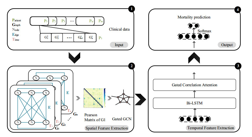
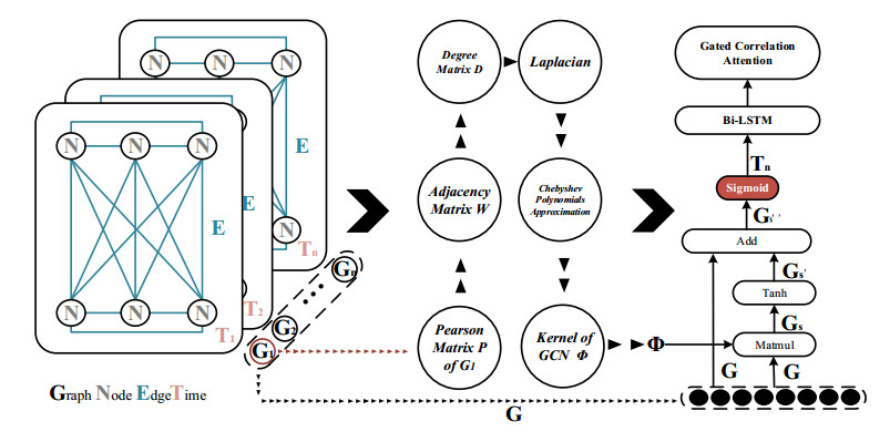
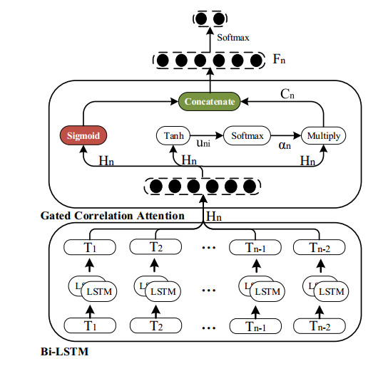
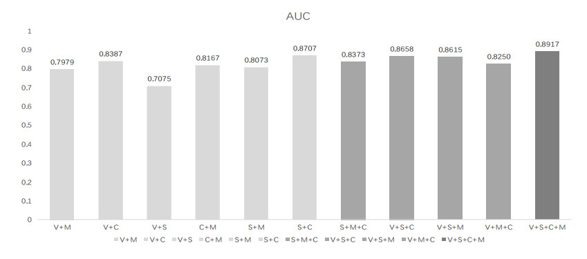
Stroke continues to be the most common cause of death in China. It has great significance for mortality prediction for stroke patients, especially in terms of analyzing the complex interactions between non-negligible factors. In this paper, we present a gated spatio-temporal correlation network (GSTCNet) to predict the one-year post-stroke mortality. Based on the four categories of risk factors: vascular event, chronic disease, medical usage and surgery, we designed a gated correlation graph convolution kernel to capture spatial features and enhance the spatial correlation between feature categories. Bi-LSTM represents the temporal features of five timestamps. The novel gated correlation attention mechanism is then connected to the Bi-LSTM to realize the comprehensive mining of spatio-temporal correlations. Using the data on 2275 patients obtained from the neurology department of a local hospital, we constructed a series of sequential experiments. The experimental results show that the proposed model achieves competitive results on each evaluation metric, reaching an AUC of 89.17%, a precision of 97.75%, a recall of 95.33% and an F1-score of 95.19%. The interpretability analysis of the feature categories and timestamps also verified the potential application value of the model for stroke.
Citation: Shuo Zhang, Yonghao Ren, Jing Wang, Bo Song, Runzhi Li, Yuming Xu. GSTCNet: Gated spatio-temporal correlation network for stroke mortality prediction[J]. Mathematical Biosciences and Engineering, 2022, 19(10): 9966-9982. doi: 10.3934/mbe.2022465
Stroke continues to be the most common cause of death in China. It has great significance for mortality prediction for stroke patients, especially in terms of analyzing the complex interactions between non-negligible factors. In this paper, we present a gated spatio-temporal correlation network (GSTCNet) to predict the one-year post-stroke mortality. Based on the four categories of risk factors: vascular event, chronic disease, medical usage and surgery, we designed a gated correlation graph convolution kernel to capture spatial features and enhance the spatial correlation between feature categories. Bi-LSTM represents the temporal features of five timestamps. The novel gated correlation attention mechanism is then connected to the Bi-LSTM to realize the comprehensive mining of spatio-temporal correlations. Using the data on 2275 patients obtained from the neurology department of a local hospital, we constructed a series of sequential experiments. The experimental results show that the proposed model achieves competitive results on each evaluation metric, reaching an AUC of 89.17%, a precision of 97.75%, a recall of 95.33% and an F1-score of 95.19%. The interpretability analysis of the feature categories and timestamps also verified the potential application value of the model for stroke.

| [1] |
Y. Wang, Z. Li, H. Gu, Y. Zhai, Y. Jiang, X. Zhao, et al., China stroke statistics 2019: A report from the national center for healthcare quality management in neurological diseases, China national clinical research center for neurological diseases, the Chinese stroke association, national center for chronic and non-communicable disease control and prevention, Chinese center for disease control and prevention and institute for global neuroscience and stroke collaborations, Stroke Vasc. Neurol., 5 (2020), 211-369.https://doi.org/10.1136/svn-2020-000457 doi: 10.1136/svn-2020-000457

|
| [2] |
S. Wu, B. Wu, M. Liu, Z. Chen, W. Wang, C. S. Anderson, et al., Stroke in China: advances and challenges in epidemiology, prevention, and management, Lancet Neurol., 18 (2019), 394-405.https://doi.org/10.1016/S1474-4422(18)30500-3 doi: 10.1016/S1474-4422(18)30500-3
|
| [3] |
T. Guan, J. Ma, M. Li, T. Xue, Z. Lan, J. Guo, et al., Rapid transitions in the epidemiology of stroke and its risk factors in China from 2002 to 2013, Neurology, 89 (2017), 53-61. httpss://doi.org/10.1212/WNL.0000000000004056 doi: 10.1212/WNL.0000000000004056
|
| [4] |
P. Zhou, J. Liu, L. Wang, W. Feng, Z. Cao, P. Wang, et al., Association of small dense low-density lipoprotein cholesterol with stroke risk, severity and prognosis, J. Atheroscler. Thromb., 27 (2020), 1310-1324.https://doi.org/10.5551/jat.53132 doi: 10.5551/jat.53132
|
| [5] |
S. Schönenberger, P. L. Hendén, C. Z. Simonsen, L. Uhlmann, C. Klose, J. A. R. Pfaff, et al., Association of general anesthesia vs procedural sedation with functional outcome among patients with acute ischemic stroke undergoing thrombectomy: a systematic review and meta-analysis, JAMA-J. Am. Med. Assoc., 322 (2019), 1283-1293.https://doi.org/10.1001/jama.2019.11455 doi: 10.1001/jama.2019.11455
|
| [6] |
C. C. Hu, A. Low, E. O'Connor, P. Siriratnam, C. Hair, T. Kraemer, et al., Diabetes in ischaemic stroke in a regional Australian hospital - uncharted territory, Intern. Med. J., 52 (2020), 574-580.https://doi.org/10.1111/imj.15073 doi: 10.1111/imj.15073
|
| [7] |
J. Xiang, H. Li, J. Xiong, F. Hua, S. Huang, Y. Jiang, et al., Acupuncture for post-stroke insomnia: A protocol for systematic review and meta-analysis, Medicine, 99 (2020), e21381.https://doi.org/10.1097/MD.0000000000021381 doi: 10.1097/MD.0000000000021381
|
| [8] |
Y. Ou, S. Sun, H. Gan, R. Zhou, Z. Yang. An improved self-supervised learning for EEG classification, Math. Biosci. Eng., 19 (2022), 6907-6922.https://doi.org/10.3934/mbe.2022325 doi: 10.3934/mbe.2022325
|
| [9] |
R. Elham, A. Hesham, A bag-of-words feature engineering approach for assessing health conditions using accelerometer data, Smart Health, 16 (2020), 100116.https://doi.org/10.1016/j.smhl.2020.100116 doi: 10.1016/j.smhl.2020.100116
|
| [10] |
Z. Zhang, Z. Ji, Q. Chen, S. Yuan, W. Fan, Joint optimization of cycleGAN and CNN classifier for detection and localization of retinal pathologies on color fundus photographs, IEEE J. Biomed. Health, 26 (2022), 115-126.https://doi.org/10.1109/JBHI.2021.3092339. doi: 10.1109/JBHI.2021.3092339
|
| [11] |
X. Zhang, Y. Hu, Z. Xiao, J. Fang, R. Higashita, J. Liu, Machine learning for cataract classification/grading on ophthalmic imaging modalities: A survey. Mach. Intell. Res., 19 (2022), 184-208.https://doi.org/10.1007/s11633-022-1329-0 doi: 10.1007/s11633-022-1329-0
|
| [12] |
Y. S. Baek, S. C. Lee, W. I. Choi, H. H. Kim, Prediction of atrial fibrillation from normal ECG using artificial intelligence in patients with unexplained stroke, Eur. Heart J., 41 (2020), ehaa946.0348.https://doi.org/10.1093/ehjci/ehaa946.0348 doi: 10.1093/ehjci/ehaa946.0348
|
| [13] |
S. Liu, X. Wang, Y. Xiang, H. Xu, H. Wang, B. Tang, Multi-channel fusion LSTM for medical event prediction using EHRs, J. Biomed. Inf., 127 (2022), 104011.https://doi.org/10.1016/j.jbi.2022.104011 doi: 10.1016/j.jbi.2022.104011
|
| [14] |
S. Zhang, J. Wang, L. Pei, K. Liu, Y. Gao, H. Fang, et al., Interpretability analysis of one-Year mortality prediction for stroke patients based on deep neural network, IEEE J. Biomed. Health, 26 (2022), 1903-1910.https://doi.org/10.1109/JBHI.2021.3123657 doi: 10.1109/JBHI.2021.3123657
|
| [15] |
S. Cheng, Q Xu, Z. Xu, Y. Shi, Y. Liu, Z. Li, et al., Effect of prior stroke on stroke outcomes in patients with Ischemic cerebrovascular disease, Chin. J. Stroke, 16 (2021), 1242-1247.https://doi.org/10.3969/j.issn.1673-5765.2021.12.008 doi: 10.3969/j.issn.1673-5765.2021.12.008
|
| [16] |
E. C. Leira, K. C. Chang, P. H. Davis, W. R. Clarke, R. F. Woolson, M. D. Hansen, et al., Can we predict early recurrence in acute stroke?, Cerebrovasc. Dis., 18 (2014), 139-144.https://doi.org/10.1159/000079267 doi: 10.1159/000079267
|
| [17] |
H. Ay, L. Gungor, E. M. Arsavae, J. Rosand, M. Vangel, T. Benner, et al., A score to predict early risk of recurrence after ischemic stroke, Neurology, 74 (2010), 128.https://doi.org/10.1212/WNL.0b013e3181ca9cff doi: 10.1212/WNL.0b013e3181ca9cff
|
| [18] |
W. N. Kernan, C. M. Viscoli, L. M. Brass, R. W. Makuch, P. M. Sarrel, R. S. Roberts, et al., The stroke prognosis instrument ii (spi-ii): A clinical pre-diction instrument for patients with transient ischemia and nondisabling ischemic stroke, Stroke, 31 (2000), 456-462.https://doi.org/10.1161/01.STR.31.2.456 doi: 10.1161/01.STR.31.2.456
|
| [19] |
CAPRIE Steering Committee, A randomised, blinded, trial of clopidogrel versus aspirin in patients at risk of ischaemic events (CAPRIE), Lancet, 348 (1996), 1329-1339.https://doi.org/10.1016/s0140-6736(96)09457-3 doi: 10.1016/s0140-6736(96)09457-3
|
| [20] |
E. M. Arsava, G. Kim, J. Oliveira-Filho, L. Gungor, H. J. Noh, M. Lordelo, et al., Prediction of early recurrence after acute ischemic stroke, JAMA Neurol., 73 (2016), 396-401.https://doi.org/10.1001/jamaneurol.2015.4949 doi: 10.1001/jamaneurol.2015.4949
|
| [21] |
L. C. Hung, S. F. Sung, Y. H. Hu, A machine learning approach to predicting readmission or mortality in patients hospitalized for stroke or transient ischemic attack, Appl. Sci., 10 (2020), 6337.https://doi.org/10.3390/app10186337 doi: 10.3390/app10186337
|
| [22] |
A. D. Jamthikar, D. Gupta, L. E. Mantella, L. Saba, J. R. Laird, A. M. Johri, et al., Multiclass machine learning vs. conventional calculators for stroke/CVD risk assessment using carotid plaque predictors with coronary angiography scores as gold standard: A 500 participants study, Int. J. Cardiovas. Imag., 37 (2021), 1171-1187.https://doi.org/10.1007/s10554-020-02099-7 doi: 10.1007/s10554-020-02099-7
|
| [23] |
J. N. Heo, J. G. Yoon, H. Park, Y. D. Kim, H. S. Nam, J. H. Heo, Machine learning based model for prediction of outcomes in acute stroke, Stroke, 50 (2019), 1263-1265.https://doi.org/10.1161/STROKEAHA.118.024293 doi: 10.1161/STROKEAHA.118.024293
|
| [24] |
C. Jiang, T. Chen, X. Du, X. Li, L. He, Y. Lai, et al., A simple and easily implemented risk model to predict 1-year ischemic stroke and systemic embolism in Chinese patients with atrial fibrillation, Chin. Med. J. -Peking, 134 (2021), 6.https://doi.org/10.1097/CM9.0000000000001515 doi: 10.1097/CM9.0000000000001515
|
| [25] |
X. Zhang, Z. Xiao, H. Fu, Y. Hu, J. Yuan, Y. Xu, et al., Attention to region: Region-based integration-and-recalibration networks for nuclear cataract classification using AS-OCT images, Med. Image Anal., 80 (2022), 102499.https://doi.org/10.1016/j.media.2022.102499 doi: 10.1016/j.media.2022.102499
|
| [26] |
Y. Su, Y. Shi, W. Lee, L. Cheng, H. Guo, TAHDNet: Time-aware hierarchical dependency network for medication recommendation, J. Biomed. Inf., 129 (2022), 104069.https://doi.org/10.1016/j.jbi.2022.104069 doi: 10.1016/j.jbi.2022.104069
|
| [27] |
X. Zhang, Z. Xiao, L. Hu, G. Xu, R. Higashita, W. Chen, et al., CCA-Net: Clinical-awareness attention network for nuclear cataract classification in AS-OCT, Knowl. -Based Syst., 250 (2022), 109109.https://doi.org/10.1016/j.knosys.2022.109109 doi: 10.1016/j.knosys.2022.109109
|
| [28] |
S. Zhang, S. Xu, L. Tan, H. Wang, J. Meng, Stroke lesion detection and analysis in MRI images based on deep learning, J. Healthc. Eng., 5 (2021), 1-9.https://doi.org/10.1155/2021/5524769 doi: 10.1155/2021/5524769
|
| [29] |
S. Zhang, J. Wang, L. Pei, K. Liu, Y. Gao, H. Fang, et al., Interpretable CNN for ischemic stroke subtype classification with active model adaptation, BMC Med. Inf. Decis., 22 (2022), 3.https://doi.org/10.1186/s12911-021-01721-5 doi: 10.1186/s12911-021-01721-5
|
| [30] |
L. Hokkinen, T. Mkel, S. Savolainen, M. Kangasniemi, Evaluation of a CTA-based convolutional neural network for infarct volume prediction in anterior cerebral circulation ischaemic stroke, Eur. Radiol. Exp., 5 (2021), 25.https://doi.org/10.1186/s41747-021-00225-1 doi: 10.1186/s41747-021-00225-1
|
| [31] | P. Chantamit-O-Pas, M. Goyal. Long short-term memory recurrent neural network for stroke prediction, in Proceeding of the Machine Learning and Data Mining in Pattern Recognition (MLDM), 2018,312-323.https://doi.org/10.1007/978-3-319-96136-1_25 |
| [32] |
L. Chen, B. Gu, Z. Wang, L. Zhang, M. Xu, S. Liu, et al., EEG-controlled functional electrical stimulation rehabilitation for chronic stroke: system design and clinical application, Front. Med. -PRC, 15 (2021), https://doi.org/10.1007/s11684-020-0794-5 doi: 10.1007/s11684-020-0794-5
|
| [33] |
Q. Li, X. Chai, C. Zhang, X. Wang, W. Ma, Prediction model of ischemic stroke recurrence using PSO-LSTM in mobile medical monitoring system, Comput. Intel. Neurosci., 2022 (2022), 8936103.https://doi.org/10.1155/2022/8936103 doi: 10.1155/2022/8936103
|
| [34] |
M. Jian, J. Wang, H. Yu, G. Wang, Integrating object proposal with attention networks for video saliency detection, Inf. Sci., 576 (2021), 819-830.https://doi.org/10.1016/j.ins.2021.08.069 doi: 10.1016/j.ins.2021.08.069
|
| [35] |
M. Jian, J. Wang, H. Yu, G. Wang, X. Meng, L. Yang, et al., Visual saliency detection by integrating spatial position prior of object with background cues, Exp. Syst. Appl., 168 (2021), 114219.https://doi.org/10.1016/j.eswa.2020.114219 doi: 10.1016/j.eswa.2020.114219
|
| [36] | T. N. Kipf, M. Welling, Semi-supervised classification with graph convolutional networks, in Proceeding of 2017 International Conference on Learning Representations (ICLR), 2017.https://doi.org/10.1145/3097983.3097997 |
| [37] |
B. Chen, J. Li, G. Lu, H. Yu, D. Zhang, Label co-occurrence learning with graph convolutional networks for multi-label chest X-Ray image classification, IEEE J. Biomed. Health, 24 (2020), 2292-2302.https://doi.org/10.1109/JBHI.2020.2967084 doi: 10.1109/JBHI.2020.2967084
|
| [38] |
E. El-allaly, M. Sarrouti, N. En-Nahnahi, S. O. E. Alaoui, An attentive joint model with transformer-based weighted graph convolutional network for extracting adverse drug event relation, J. Biomed. Inf., 125 (2022), 103968.https://doi.org/10.1016/j.jbi.2021.103968 doi: 10.1016/j.jbi.2021.103968
|
| [39] |
W. Peng, T. Chen, W. Dai, Predicting drug response based on multi-omics fusion and graph convolution, IEEE J. Biomed. Health, 26 (2022), 1384-1393.https://doi.org/10.1109/JBHI.2021.3102186 doi: 10.1109/JBHI.2021.3102186
|
| [40] |
C. Mao, L. Yao, Y. Luo, MedGCN: Medication recommendation and lab test imputation via graph convolutional networks, J. Biomed. Inf., 127 (2022), 104000.https://doi.org/10.1016/j.jbi.2022.104000 doi: 10.1016/j.jbi.2022.104000
|
Figures(5) / Tables(7)

Shuo Zhang, Yonghao Ren, Jing Wang, Bo Song, Runzhi Li, Yuming Xu. GSTCNet: Gated spatio-temporal correlation network for stroke mortality prediction[J]. Mathematical Biosciences and Engineering, 2022, 19(10): 9966-9982. doi: 10.3934/mbe.2022465


 DownLoad: