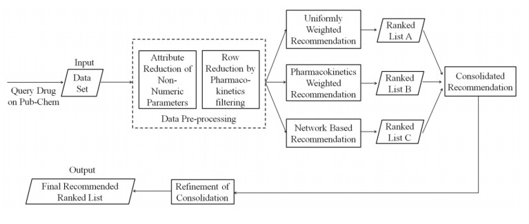
Tuberculosis (TB) is a fatal infectious disease which affected millions of people worldwide for many decades and now with mutating drug resistant strains, it poses bigger challenges in treatment of the patients. Computational techniques might play a crucial role in rapidly developing new or modified anti-tuberculosis drugs which can tackle these mutating strains of TB. This research work applied a computational approach to generate a unique recommendation list of possible TB drugs as an alternate to a popular drug, EMB, by first securing an initial list of drugs from a popular online database, PubChem, and thereafter applying an ensemble of ranking mechanisms. As a novelty, both the pharmacokinetic properties and some network based attributes of the chemical structure of the drugs are considered for generating separate recommendation lists. The work also provides customized modifications on a popular and traditional ensemble ranking technique to cater to the specific dataset and requirements. The final recommendation list provides established chemical structures along with their ranks, which could be used as alternatives to EMB. It is believed that the incorporation of both pharmacokinetic and network based properties in the ensemble ranking process added to the effectiveness and relevance of the final recommendation.
Citation: Rishin Haldar, Swathi Jamjala Narayanan. A novel ensemble based recommendation approach using network based analysis for identification of effective drugs for Tuberculosis[J]. Mathematical Biosciences and Engineering, 2022, 19(1): 873-891. doi: 10.3934/mbe.2022040
Tuberculosis (TB) is a fatal infectious disease which affected millions of people worldwide for many decades and now with mutating drug resistant strains, it poses bigger challenges in treatment of the patients. Computational techniques might play a crucial role in rapidly developing new or modified anti-tuberculosis drugs which can tackle these mutating strains of TB. This research work applied a computational approach to generate a unique recommendation list of possible TB drugs as an alternate to a popular drug, EMB, by first securing an initial list of drugs from a popular online database, PubChem, and thereafter applying an ensemble of ranking mechanisms. As a novelty, both the pharmacokinetic properties and some network based attributes of the chemical structure of the drugs are considered for generating separate recommendation lists. The work also provides customized modifications on a popular and traditional ensemble ranking technique to cater to the specific dataset and requirements. The final recommendation list provides established chemical structures along with their ranks, which could be used as alternatives to EMB. It is believed that the incorporation of both pharmacokinetic and network based properties in the ensemble ranking process added to the effectiveness and relevance of the final recommendation.

| [1] |
V. Eldholm, J. Monteserin, A. Rieux, B. Lopez, B. Sobkowiak, V. Ritacco, et al., Four decades of transmission of a multidrug-resistant Mycobacterium tuberculosis outbreak strain, Nat. Comm., 6 (2015), 1–9. doi: 10.1038/ncomms8119. doi: 10.1038/ncomms8119

|
| [2] |
J. D. Fonseca, G. M. Knight, T. D. McHugh, The complex evolution of antibiotic resistance in Mycobacterium tuberculosis, Int. J. Infect. Dis., 32 (2015), 94–100. doi: 10.1016/j.ijid.2015.01.014. doi: 10.1016/j.ijid.2015.01.014
|
| [3] |
B. Müller, S. Borrell, G. Rose, S. Gagneux, The heterogeneous evolution of multidrug-resistant Mycobacterium tuberculosis, Trends Genet., 29 (2013), 160–169. doi: 10.1016/j.tig.2012.11.005. doi: 10.1016/j.tig.2012.11.005
|
| [4] |
S. Ekins, J. S. Freundlich, I. Choi, M. Sarker, C. Talcott, Computational databases, pathway and cheminformatics tools for tuberculosis drug discovery, Trends Microb., 19 (2011), 65–74. doi: 10.1016/j.tim.2010.10.005. doi: 10.1016/j.tim.2010.10.005
|
| [5] |
A. Sandgren, M. Strong, P. Muthukrishnan, B. K. Weiner, G. M. Church, M. B. Murray, Tuberculosis drug resistance mutation database, PLoS Med., 6 (2009), e1000002. doi: 10.1371/journal.pmed.1000002. doi: 10.1371/journal.pmed.1000002
|
| [6] |
L. Chen, Z. Xiong, L. Sun, J. Yang, Q. Jin, VFDB 2012 update: Toward the genetic diversity and molecular evolution of bacterial virulence factors, Nucleic Acids Res., 40 (2012), 641–645. doi: 10.1093/nar/gkr989. doi: 10.1093/nar/gkr989
|
| [7] |
S. Kim, J. Chen, T. Cheng, A. Gindulyte, J. He, S. He, Q. Li et al., PubChem 2019 update: Improved access to chemical data, Nucleic Acids Res., 47 (2019), 1102–1109. doi: 10.1093/nar/gky1033. doi: 10.1093/nar/gky1033
|
| [8] |
R. C. Goldman, Target discovery for new antitubercular drugs using a large dataset of growth inhibitors from PubChem, Infect. Dis.-Drug Tar., 20 (2020), 352–366. doi: 10.2174/1871526519666181205163810. doi: 10.2174/1871526519666181205163810
|
| [9] |
C. A. Lipinski, F. Lombardo, B. W. Dominy, P. J. Feeney, Experimental and computational approaches to estimate solubility and permeability in drug discovery and development settings, Adv. Drug Deliv. Rev., 23 (1997), 3–25. doi: 10.1016/s0169-409x(96)00423-1. doi: 10.1016/s0169-409x(96)00423-1
|
| [10] |
S. Ekins, J. S. Freundlich, R. C. Reynolds, Fusing dual-event data sets for Mycobacterium tuberculosis machine learning models and their evaluation, J. Chem. Info. Model., 53 (2013), 3054–3063. doi: 10.1021/ci400480s. doi: 10.1021/ci400480s
|
| [11] |
S. Ekins, A. C. Casey, D. Roberts, T. Parish, B. A. Bunin, Bayesian models for screening and TB Mobile for target inference with Mycobacterium tuberculosis, Tuberculosis, 94 (2014), 162–169. doi: 10.1016/j.tube.2013.12.001. doi: 10.1016/j.tube.2013.12.001
|
| [12] |
S. Ekins, A. M. Clark, S. J. Swamidass, N. Litterman, A. J. Williams, Bigger data, collaborative tools and the future of predictive drug discovery, J. Computer-aided Mol. Des., 28 (2014), 997–1008. doi: 10.1007/s10822-014-9762-y. doi: 10.1007/s10822-014-9762-y
|
| [13] |
S. Ekins, A. M. Clark, A. L. Perryman, J. S. Freundlich, A. Korotcov, V. Tkachenko, Accessible machine learning approaches for toxicology, Comp. Tox. Risk Assess Chem., (2018), 1–29. doi: 10.1002/9781119282594.ch1. doi: 10.1002/9781119282594.ch1
|
| [14] |
K. Djaout, V. Singh, Y. Boum, V. Katawera, H. F. Becker, N. G. Bush, et al., Predictive modeling targets thymidylate synthase ThyX in Mycobacterium tuberculosis, Sci. Rep., 6 (2016), 1–11. doi: 10.1038/srep27792. doi: 10.1038/srep27792
|
| [15] |
S. Chetty, M. Ramesh, A. Singh-Pillay, M. E. S. Soliman, Recent advancements in the development of anti-tuberculosis drugs, Bioorg. Med. Chem. Let., 27 (2017), 370–386. doi: 10.1016/j.bmcl.2016.11.084. doi: 10.1016/j.bmcl.2016.11.084
|
| [16] |
D. Machado, M. Girardini, M. Viveiros, M. Pieroni, Challenging the drug-likeness dogma for new drug discovery in tuberculosis, Front. Microbio., 9 (2018), 1367. doi: 10.3389/fmicb.2018.01367. doi: 10.3389/fmicb.2018.01367
|
| [17] |
M. AlMatar, H. AlMandeal, I. Var, B. Kayar, F. Köksal, New drugs for the treatment ofMycobacterium tuberculosis infection, Biomed. Pharmaco., 91 (2017), 546–558. doi: 10.1016/j.biopha.2017.04.105. doi: 10.1016/j.biopha.2017.04.105
|
| [18] |
L. D. Ghiraldi-Lopes, P. A. Z. Campanerut-Sá, G. P. C. Evaristo, J. E. Meneguello, A. Fiorini, V. P. Baldin, et al., New insights on Ethambutol Targets in Mycobacterium tuberculosis, Infect. Dis.-Drug Tar., 19 (2019), 73–80. doi: 10.2174/1871526518666180124140840. doi: 10.2174/1871526518666180124140840
|
| [19] | S. L. Kinnings, N. Liu, N. Buchmeier, P. J. Tonge, L. Xie, P. E. Bourne, Drug discovery using chemical systems biology: Repositioning the safe medicine Comtan to treat multi-drug and extensively drug resistant tuberculosis, PLoS Comp. Biol., 5 (2009), e1000423. doi; 10.1371/journal.pcbi.1000423. |
| [20] | J. T. Dudley, T. Deshpande, A. J. Butte, Exploiting drug–disease relationships for computational drug repositioning, Brief Bioinfo., 12 (2011), 303–311. doi; 10.1093/bib/bbr013. |
| [21] |
A. Maitra, S. Bates, T. Kolvekar, P. V. Devarajan, J. D. Guzman, S. Bhakta, Repurposing—a ray of hope in tackling extensively drug resistance in tuberculosis, Int. J. Inf. Dis., 32 (2015), 50–55. doi: 10.1016/j.ijid.2014.12.031. doi: 10.1016/j.ijid.2014.12.031
|
| [22] |
Q. Vanhaelen, P. Mamoshina, A. M. Aliper, A. Artemov, K. Lezhnina, I. Ozerov, et al., Design of efficient computational workflows for in silico drug repurposing, Drug Disco. Tod., 22 (2017), 210–222. doi: 10.1016/j.drudis.2016.09.019. doi: 10.1016/j.drudis.2016.09.019
|
| [23] |
E. March-Vila, L. Pinzi, N. Sturm, A. Tinivella, O. Engkvist, H. Chen, et al., On the integration of in silico drug design methods for drug repurposing, Front. Pharma., 8 (2017), 298. doi: 10.3389/fphar.2017.00298. doi: 10.3389/fphar.2017.00298
|
| [24] |
K. Pavić, I. Perković, Š. Pospíšilová, M. Machado, D. Fontinha, M. Prudêncio, et al., Primaquine hybrids as promising antimycobacterial and antimalarial agents, Euro. J. Med. Chem., 143 (2018), 769–779. doi: 10.1016/j.ejmech.2017.11.083. doi: 10.1016/j.ejmech.2017.11.083
|
| [25] |
A. C. Pushkaran, V. Vinod, M. Vanuopadath, S. S. Nair, S. V. Nair, A. K. Vasudevan, et al., Combination of repurposed drug diosmin with amoxicillin-clavulanic acid causes synergistic inhibition of mycobacterial growth, Sci. Rep., 9 (2019), 1–14. doi: 10.1038/s41598-019-43201-x. doi: 10.1038/s41598-019-43201-x
|
| [26] |
J. V. Eichborn, M. S. Murgueitio, M. Dunkel, S. Koerner, P. E. Bourne, R. Preissner, PROMISCUOUS: A database for network-based drug-repositioning, Nucleic Acids Res., 39 (2010), 1060–1066. doi: 10.1093/nar/gkq1037. doi: 10.1093/nar/gkq1037
|
| [27] |
S. Hasan, B. K. Bonde, N. S. Buchan, M. D. Hall, Network analysis has diverse roles in drug discovery, Drug Disc. Tod., 17 (2012), 869–874. doi: 10.1016/j.drudis.2012.05.006. doi: 10.1016/j.drudis.2012.05.006
|
| [28] |
S. Daminelli, V. J. Haupt, M. Reimann, M. Schroeder, Drug repositioning through incomplete bi-cliques in an integrated drug–target–disease network, Integ. Biol., 4 (2012), 778–788. doi: 10.1039/c2ib00154c. doi: 10.1039/c2ib00154c
|
| [29] |
N. Chandra, J. Padiadpu, Network approaches to drug discovery, Expert Op. Drug Disc., 8 (2013), 7–20. doi: 10.1517/17460441.2013.741119. doi: 10.1517/17460441.2013.741119
|
| [30] |
B. K. Chung, T. Dick, D. Lee, In silico analyses for the discovery of tuberculosis drug targets, J. Antimicro. Chemo., 68 (2013), 2701–2709. doi: 10.1093/jac/dkt273. doi: 10.1093/jac/dkt273
|
| [31] |
Z. Wu, Y. Wang, L. Chen, Network-based drug repositioning, Mol. BioSys., 9 (2013), 1268–1281. doi: 10.1039/c3mb25382a. doi: 10.1039/c3mb25382a
|
| [32] |
P. Anand, N. Chandra, Characterizing the pocketome of Mycobacterium tuberculosis and application in rationalizing polypharmacological target selection, Sci. Rep., 4 (2014), 1–17. doi: 10.1038/srep06356. doi: 10.1038/srep06356
|
| [33] |
E. Guney, J. Menche, M. Vidal, A. Barábasi, Network-based in silico drug efficacy screening, Nat.Comm., 7 (2016), 1–13. doi: 10.1038/ncomms10331. doi: 10.1038/ncomms10331
|
| [34] |
P. Emerson, The original Borda count and partial voting, Soc. Choice Welf., 40 (2013), 353–358. doi: 10.1007/s00355-011-0603-9. doi: 10.1007/s00355-011-0603-9
|
| [35] |
J. Fraenkel, B. Grofman, The Borda Count and its real-world alternatives: Comparing scoring rules in Nauru and Slovenia, Australian J. Pol. Sc., 49 (2014), 186–205. doi: 10.1080/10361146.2014.900530. doi: 10.1080/10361146.2014.900530
|
| [36] |
M. H. Alsharif, Y. H. Alsharif, S. A. Chaudhry, M. A. Albreem, A. Jahid, E. Hwang, Artificial intelligence technology for diagnosing COVID-19 cases: A review of substantial issues, Eur. Rev. Med. Pharmacol. Sci., 24 (2020), 9226–9233. doi: 10.26355/eurrev_202009_22875. doi: 10.26355/eurrev_202009_22875
|
| [37] |
M. H. Alsharif, Y. H. Alsharif, M. A. Albreem, A. Jahid, A. A. A. Solyman, K. Yahya, et al., Application of machine intelligence technology in the detection of vaccines and medicines for SARS-CoV-2, Eur. Rev. Med. Pharmacol. Sci., 24 (2020), 11977–11981. doi: 10.26355/eurrev_202011_23860. doi: 10.26355/eurrev_202011_23860
|
| [38] |
M. H. Alsharif, Y. H. Alsharif, K. Yahya, O. A. Alomari, M. A. Albreem, A. Jahid, Deep learning applications to combat the dissemination of COVID-19 disease: A review, Eur. Rev. Med. Pharmacol. Sci., 24 (2020), 11455–11460. doi: 10.26355/eurrev_202011_23640. doi: 10.26355/eurrev_202011_23640
|
| [39] |
G. Elmas, A. Okumuş, R. Cemaloğlu, Z. Kılıç, S. P. Çelik, L. Açık, et al., Phosphorus-nitrogen compounds. part 38. Syntheses, characterizations, cytotoxic, antituberculosis and antimicrobial activities and DNA interactions of spirocyclotetraphosphazenes with bis-ferrocenyl pendant arms, J. Organomet. Chem., 853 (2017), 93–106. doi: 10.1016/j.jorganchem.2017.10.025. doi: 10.1016/j.jorganchem.2017.10.025
|
| [40] |
K. Tahlan, R. Wilson, D. B. Kastrinsky, K. Arora, V. Nair, E. Fischer, et al., SQ109 targets MmpL3, a membrane transporter of trehalose monomycolate involved in mycolic acid donation to the cell wall core of Mycobacterium tuberculosis, Antimicro. Agents Chemo., 56 (2012), 1797–1809. doi: 10.1128/AAC.05708-11. doi: 10.1128/AAC.05708-11
|
| [41] | M. A. Musa, V. L. D. Badisa, L. M. Latinwo, Cytotoxic activity of N, N'-Bis (2-hydroxybenzyl) ethylenediamine derivatives in human cancer cell lines, Anticancer Res., 34 (2014), 1601–1607. |

Figures(3) / Tables(6)

Rishin Haldar, Swathi Jamjala Narayanan. A novel ensemble based recommendation approach using network based analysis for identification of effective drugs for Tuberculosis[J]. Mathematical Biosciences and Engineering, 2022, 19(1): 873-891. doi: 10.3934/mbe.2022040


 DownLoad: