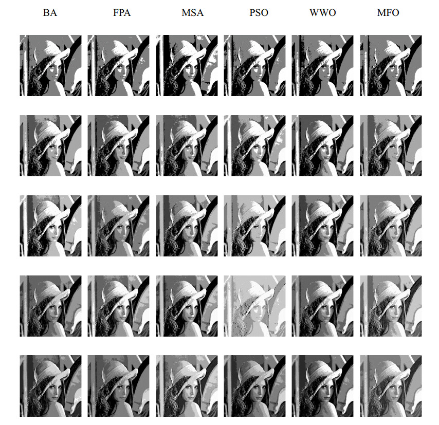
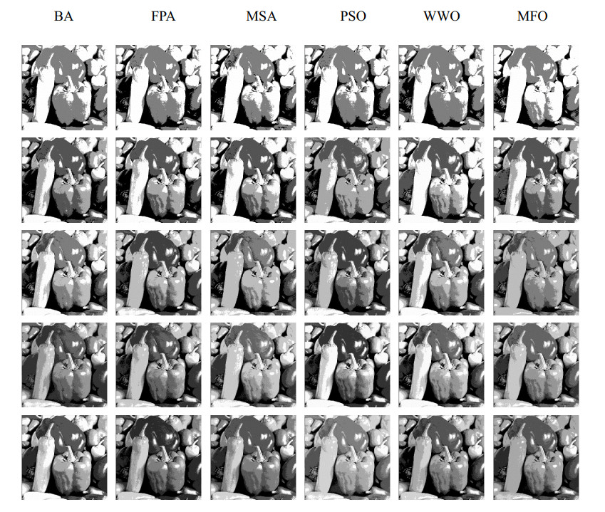
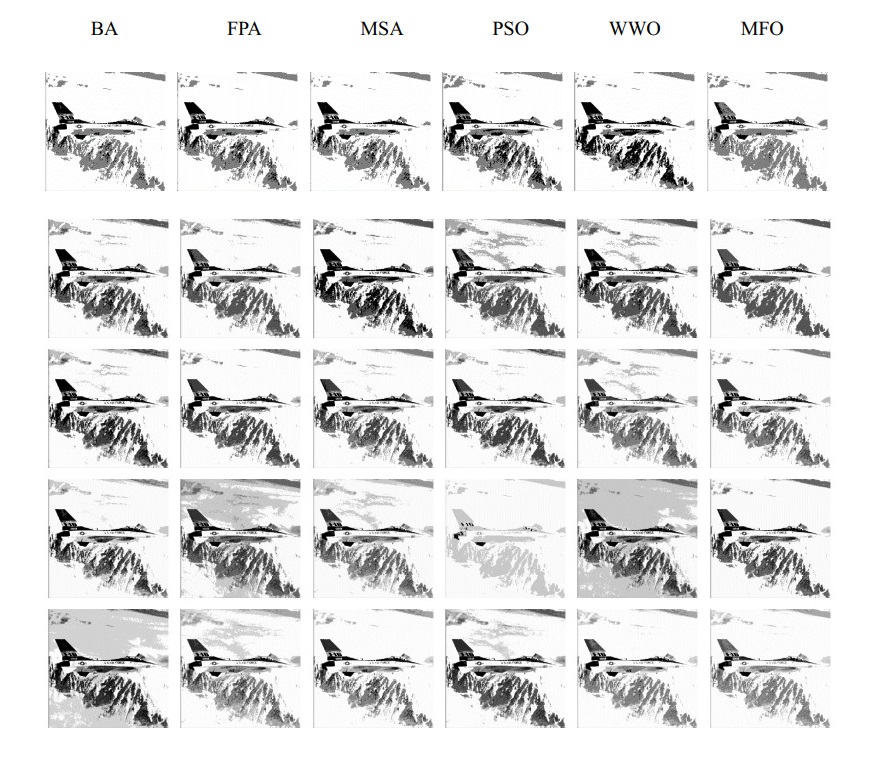
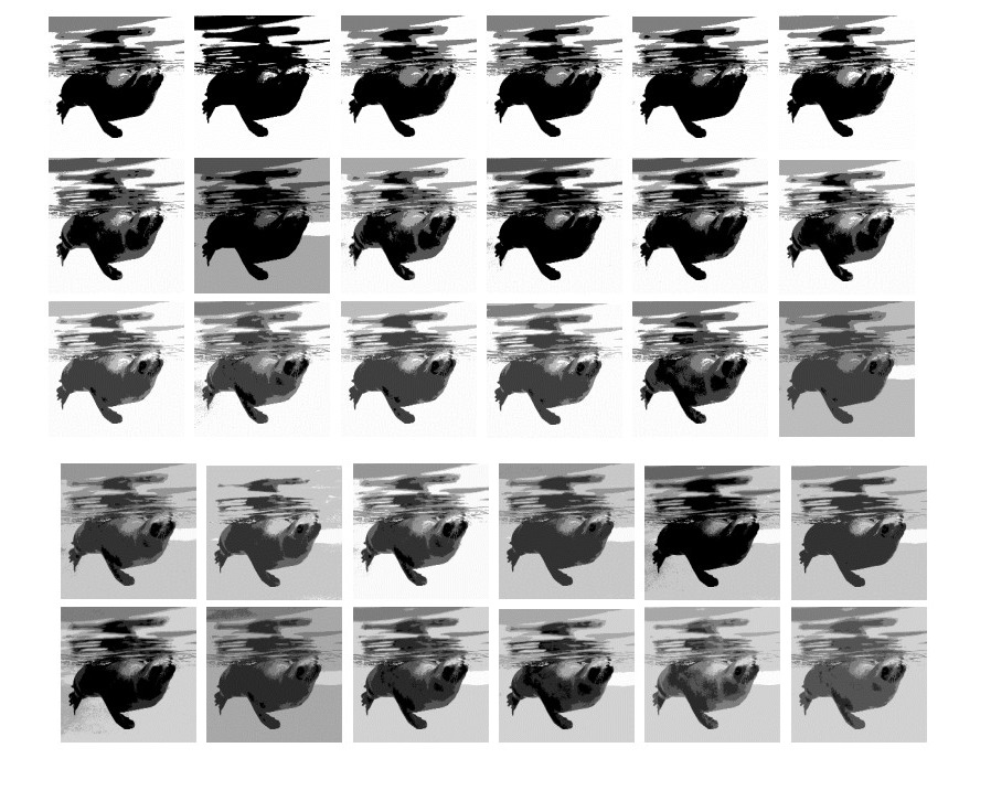
Multilevel thresholding is a reliable and efficacious method for image segmentation that has recently received widespread recognition. However, the computational complexity of the multilevel thresholding method increases as the threshold level increases, which causes the low segmentation accuracy of this method. To overcome this shortcoming, this paper presents a moth-flame optimization (MFO) established on Kapur's entropy to clarify the multilevel thresholding image segmentation. The MFO adjusts exploration and exploitation to achieve the best fitness value. To validate the overall performance, MFO is compared with other algorithms to realize the global optimal solution to maximize the target value of Kapur's entropy. Some critical evaluation indicators are used to determine the segmentation effect and optimization performance of each algorithm. The experimental results indicate that MFO has a faster convergence speed, higher calculation accuracy, better segmentation effect and better stability.
Citation: Wenqi Ji, Xiaoguang He. Kapur's entropy for multilevel thresholding image segmentation based on moth-flame optimization[J]. Mathematical Biosciences and Engineering, 2021, 18(6): 7110-7142. doi: 10.3934/mbe.2021353
Multilevel thresholding is a reliable and efficacious method for image segmentation that has recently received widespread recognition. However, the computational complexity of the multilevel thresholding method increases as the threshold level increases, which causes the low segmentation accuracy of this method. To overcome this shortcoming, this paper presents a moth-flame optimization (MFO) established on Kapur's entropy to clarify the multilevel thresholding image segmentation. The MFO adjusts exploration and exploitation to achieve the best fitness value. To validate the overall performance, MFO is compared with other algorithms to realize the global optimal solution to maximize the target value of Kapur's entropy. Some critical evaluation indicators are used to determine the segmentation effect and optimization performance of each algorithm. The experimental results indicate that MFO has a faster convergence speed, higher calculation accuracy, better segmentation effect and better stability.

| [1] | M. A. Elaziz, D. Oliva, A. A. Ewees, S. Xiong, Multi-level thresholding-based grey scale image segmentation using multi-objective multi-verse optimizer, Expert Syst. Appl., 125 (2019), 112-129. |
| [2] | K. S. Fu, J. K. Mui, A survey on image segmentation, Pattern recognit., 13 (1981), 3-16. |
| [3] | L. He, S. Huang, Modified firefly algorithm based multilevel thresholding for color image segmentation, Neurocomputing, 240 (2017), 152-174. |
| [4] | S. Hinojosa, K. G. Dhal, M. A. Elaziz, D. Oliva, E. Cuevas, Entropy-based imagery segmentation for breast histology using the Stochastic Fractal Search, Neurocomputing, 321 (2018), 201-215. |
| [5] | S. H. Lee, H. I. Koo, N. I. Cho, Image segmentation algorithms based on the machine learning of features, Pattern Recognit. Lett., 31 (2010), 2325-2336. |
| [6] | F. Breve, Interactive image segmentation using label propagation through complex network, Expert Syst. Appl., 123 (2019), 18-33. |
| [7] | W. Chen, H. Yue, J. Wang, X. Wu, An improved edge detection algorithm for depth map inpainting, Opt. Laser Eng., 55 (2014), 69-77. |
| [8] | Y. Li, X. Bai, L. Jiao, Y. Xue, Partitioned-cooperative quantum-behaved particle swarm optimization based on multilevel thresholding applied to medical image segmentation, Appl. Soft. Comput., 56 (2017), 345-356. |
| [9] | N. Tang, F. Zhou, Z. Gu, H. Zheng, Z. Yu, B. Zheng, Unsupervised pixel-wise classification for Chaetoceros image segmentation, Neurocomputing, 318 (2018), 261-270. |
| [10] | D. H. M. P. Van, S. C. De Lange, A. Zalesky, A. Zalesky, C. Seguin, B. T. Yeo, Proportional thresholding in resting-state fMRI functional connectivity networks and consequences for patient-control connectome studies: Issues and recommendations, Neuroimage, 152 (2017), 437-449. |
| [11] | X. S. Yang, X. S. He, Bat algorithm: literature review and applicationsm, Int. J. Bio-Inspired Comput., 5 (2013), 141-149. |
| [12] | X. Yang, Flower pollination algorithm for global optimization, in International Conference on Unconventional Computation, (2012), 240-249. |
| [13] | A. A. A. Mohamed, Y. S. Mohamed, A. A. Elgaafary, A. M. Hemeida, Optimal power flow using moth swarm algorithm, Electr. Power Syst. Res., 142 (2017), 190-206. |
| [14] | J. Kennedy, R. C. Eberhart, Particle Swarm Optimization, in International Conference on Networks, 4 (2002), 1942-1948. |
| [15] | Y. J. Zheng, Water wave optimization: a new nature-inspired metaheuristic, Comput. Oper. Res., 55 (2015), 1-11. |
| [16] | Z. Yan, J. Zhang, J. Tang, Modified water wave optimization algorithm for underwater multilevel thresholding image segmentation, Multimed. Tools Appl., 79 (2020), 32415-32448. |
| [17] | X. Li, J. Song, F. Zhang, X. Ouyang, S. U. Khan, MapReduce-based fast fuzzy c-means algorithm for large-scale underwater image segmentation, Future Gener. Comp. Syst., 65 (2016), 90-101. |
| [18] | X. Bao, H. Jia, C. Lang, A novel hybrid harris hawks optimization for color image multilevel thresholding segmentation, IEEE Access, 7 (2019), 76529-76546. |
| [19] | H. Gao, Z. Fu, C. M. Pun, H. Hu, R. Lan, A multi-level thresholding image segmentation based on an improved artificial bee colony algorithm, Comput. Electr. Eng., 70 (2018), 931-938. |
| [20] | B. Akay, A study on particle swarm optimization and artificial bee colony algorithms for multilevel thresholding, Appl. Soft. Comput., 13 (2013), 3066-3091. |
| [21] | S. Pare, A. Kumar, V. Bajaj, G. K. Singh, An efficient method for multilevel color image thresholding using cuckoo search algorithm based on minimum cross entropy, Appl. Soft. Comput., 61 (2017), 570-592. |
| [22] | Z. Lu, Y. Qiu, T. Zhan, Neutrosophic C-means clustering with local information and noise distance-based kernel metric image segmentation, J. Vis. Commun. Image Rep., 58 (2019), 269-276. |
| [23] | A. Galdran, D. Pardo, A. Picón, A. Alvarez-Gila, Automatic red-channel underwater image restoration, J. Vis. Commun. Image Rep., 26 (2015), 132-145. |
| [24] | S. Vasamsetti, N. Mittal, B. C. Neelapu, H. K. Sardana, Wavelet based perspective on variational enhancement technique for underwater imagery, Ocean Eng., 141 (2017), 88-100. |
| [25] | V. K. Bohat, K. V. Arya, A new heuristic for multilevel thresholding of images, Expert Syst. Appl., 117 (2019), 176-203. |
| [26] | S. Ouadfel, A. Taleb-Ahmed, Social spiders optimization and flower pollination algorithm for multilevel image thresholding: a performance study, Expert Syst. Appl., 55 (2016), 566-584. |
| [27] | S. Pare, A. K. Bhandari, A. Kumar, G. K. Singh, A new technique for multilevel color image thresholding based on modified fuzzy entropy and Lévy flight firefly algorithm, Comput. Electr. Eng., 70 (2018), 476-495. |
| [28] | S. C. Satapathy, N. S. M. Raja, V. Rajinikanth, A. S. Ashour, N. Dey, Multi-level image thresholding using Otsu and chaotic bat algorithm, Neural Comput. Appl., 29 (2018), 1285-1307. |
| [29] | S. Emberton, L. Chittka, A. Cavallaro, Underwater image and video dehazing with pure haze region segmentation, Comput. Vis. Image Underst., 168 (2018), 145-156. |
| [30] | R. K. Sambandam, S. Jayaraman, Self-adaptive dragonfly based optimal thresholding for multilevel segmentation of digital images, in Journal of King Saud University-Computer and Information Sciences, 30 (2018), 449-461. |
| [31] | G. Sun, A. Zhang, Y. Yao, Z. Wang, A novel hybrid algorithm of gravitational search algorithm with genetic algorithm for multi-level thresholding, Appl. Soft. Comput., 46 (2016), 703-730. |
| [32] | M. A. Díaz-Cortés, N. Ortega-Sánchez, S. Hinojosa, D. Oliva, E. Cuevas, R. Rojas, A. Demin, A multi-level thresholding method for breast thermograms analysis using Dragonfly algorithm, Infrared Phys. Technol., 93 (2018), 346-361. |
| [33] | L. Shen, C. Fan, X. Huang, Multi-level image thresholding using modified flower pollination algorithm, IEEE Access, 6 (2018), 30508-30519. |
| [34] | G. Hou, Z. Pan, G. Wang, H. Yang, J. Duan, An efficient nonlocal variational method with application to underwater image restoration, Neurocomputing, 369 (2019), 106-121. |
| [35] | Y. Zhou, X. Yang, Y. Ling, J. Zhang, Meta-heuristic moth swarm algorithm for multilevel thresholding image segmentation, Multimed. Tools Appl., 77 (2018), 23699-23727. |
| [36] | R. Kalyani, P. D. Sathya, V. P. Sakthivel, Multilevel thresholding for image segmentation with exchange market algorithm, Multimed. Tools Appl., 80 (2021), 27553-27591. |
| [37] | L. Duan, S. Yang, D. Zhang, Multilevel thresholding using an improved cuckoo search algorithm for image segmentation, J. Supercomput., 77 (2021), 6734-6753. |
| [38] | M. A. Elaziz, N. Nabil, R. Moghdani, A. A. Ewees, E. Cuevas, S. Lu, Multilevel thresholding image segmentation based on improved volleyball premier league algorithm using whale optimization algorithm, Multimed. Tools Appl., 80 (2021), 12435-12468. |
| [39] | L. Li, L. Sun, Y. Xue, S. Li, R. F. Mansour, Fuzzy multilevel image thresholding based on improved coyote optimization algorithm, IEEE Access, 9 (2021), 33595-33607. |
| [40] | Q. Luo, X. Yang, Y. Zhou, Nature-inspired approach: An enhanced moth swarm algorithm for global optimization, Math. Comput. Simul., 159 (2019), 57-92. |
| [41] | Z. Li, Y. Zhou, S. Zhang, J. Song, Lévy-flight moth-flame algorithm for function optimization and engineering design problems, Math. Probl. Eng., (2016), 1-22. |
| [42] | P. Wang, Y. Zhou, Q. Luo, C. Han, M. Lei, Complex-valued encoding metaheuristic optimization algorithm: A comprehensive survey, Neurocomputing, 407 (2020), 313-342. |
| [43] | S. Mirjalili, Moth-flame optimization algorithm: A novel nature-inspired heuristic paradigm, Knowledge-based Syst., 89 (2015), 228-249. |
| [44] | B. Gao, X. Q. Li, W. L. Woo, G. Y. Tian, Physics-based image segmentation using first order statistical properties and genetic algorithm for inductive thermography imaging, IEEE Trans. Image Process., 27 (2017), 2160-2175. |
| [45] | J. N. Kapur, P. K. Sahoo, A. K. C. Wong, A new method for gray-level picture thresholding using the entropy of the histogram, in Computer vision, graphics, and image processing, 29 (1985), 273-285. |
| [46] | A. Aldahdooh, E. Masala, G. Van Wallendael, M. Barkowsky, Framework for reproducible objective video quality research with case study on PSNR implementations, Digit. Signal Prog., 77 (2018), 195-206. |
| [47] | Z. Wang, A. C. Bovik, H. R. Sheikh, E. P. Simoncelli, Image quality assessment: from error visibility to structural similarity, IEEE Trans. Image Process., 13 (2004), 600-612. |
| [48] | F. Wilcoxon, Individual Comparisons by Ranking Methods, Biom. Bull., 1 (1945), 80-83. |
Figures(14) / Tables(9)

Wenqi Ji, Xiaoguang He. Kapur's entropy for multilevel thresholding image segmentation based on moth-flame optimization[J]. Mathematical Biosciences and Engineering, 2021, 18(6): 7110-7142. doi: 10.3934/mbe.2021353


 DownLoad: