Michell truss design for lightweight gear bodies

Ganjun Xu; Ning Dai; Ganjun Xu; Ning Dai

doi:10.3934/mbe.2021085

Mathematical Biosciences and Engineering

2021, Volume 18, Issue 2: 1653-1669. doi: 10.3934/mbe.2021085

Previous Article Next Article

Research article Special Issues

Michell truss design for lightweight gear bodies

Ganjun Xu ,
Ning Dai ^,

College of Mechanical and Electrical Engineering, Nanjing University of Aeronautics and Astronautics, Nanjing 210016, China

Received: 09 November 2020 Accepted: 31 January 2021 Published: 03 February 2021

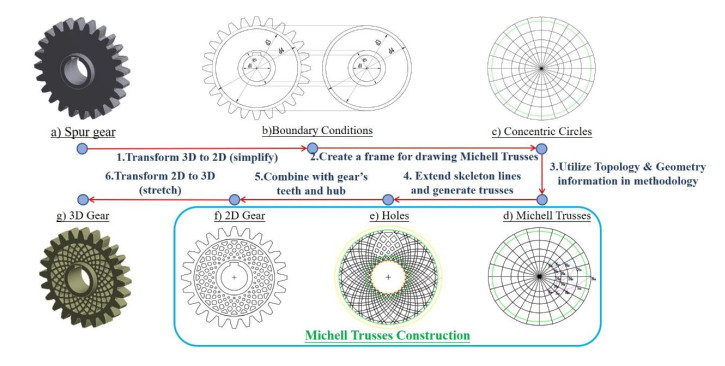
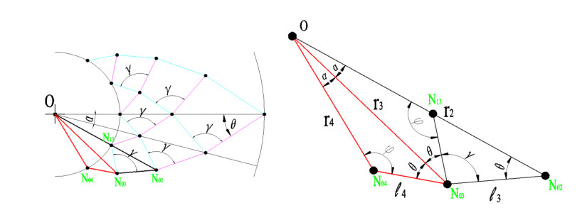
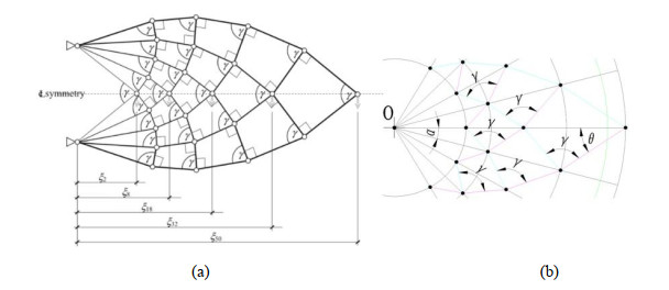
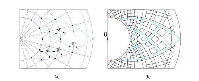
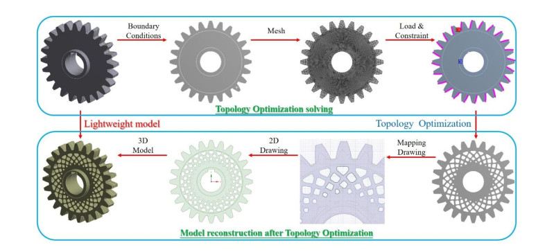
A new method for lightweight gear design based on Michell Trusses Design method was investigated in this research to compare with the traditional Topology Optimization method. A workflow with detailed steps was established using example of constructing Michell Trusses to make lightening holes at the gear's web. In this workflow, Michell Trusses are generated from a set of concentric circles. By solving the equation with the variables of concentric circles (complexity), the optimal orthogonality of trusses can be determined. Real experiments were conducted to compare the two design methods in the aspects of design costs and product mechanical property, including recording the time consumed in each link and detecting the force of failure of gears by a testing platform. The results indicate that this new method can significantly reduce design time while maintain the same power-to-weight ratio as the Topology Optimization design, which potentially provide a new research direction for lightweight structural modeling in mechanical engineering and aviation industry. The experimental product developed in this research demonstrated the promising prospects for real world applications.

Keywords:

Citation: Ganjun Xu, Ning Dai. Michell truss design for lightweight gear bodies[J]. Mathematical Biosciences and Engineering, 2021, 18(2): 1653-1669. doi: 10.3934/mbe.2021085

Related Papers:

[1]	Chaudry Masood Khalique, Kentse Maefo . A study on the (2+1)–dimensional first extended Calogero-Bogoyavlenskii- Schiff equation. Mathematical Biosciences and Engineering, 2021, 18(5): 5816-5835. doi: 10.3934/mbe.2021293
[2]	Weidong Zhao, Mobeen Munir, Ghulam Murtaza, Muhammad Athar . Lie symmetries of Benjamin-Ono equation. Mathematical Biosciences and Engineering, 2021, 18(6): 9496-9510. doi: 10.3934/mbe.2021466
[3]	Ivan Tsyfra, Wojciech Rzeszut . On reducing and finding solutions of nonlinear evolutionary equations via generalized symmetry of ordinary differential equations. Mathematical Biosciences and Engineering, 2022, 19(7): 6962-6984. doi: 10.3934/mbe.2022328
[4]	Raghu Raghavan . Growth and form, Lie algebras and special functions. Mathematical Biosciences and Engineering, 2021, 18(4): 3598-3645. doi: 10.3934/mbe.2021181
[5]	Boris Andreianov, Carlotta Donadello, Ulrich Razafison, Massimiliano D. Rosini . Riemann problems with non--local point constraints and capacity drop. Mathematical Biosciences and Engineering, 2015, 12(2): 259-278. doi: 10.3934/mbe.2015.12.259
[6]	Francesca Marcellini . The Riemann problem for a Two-Phase model for road traffic with fixed or moving constraints. Mathematical Biosciences and Engineering, 2020, 17(2): 1218-1232. doi: 10.3934/mbe.2020062
[7]	Salvador Chulián, Álvaro Martinez-Rubio, María Luz Gandarias, María Rosa . Lie point symmetries for generalised Fisher's equations describing tumour dynamics. Mathematical Biosciences and Engineering, 2021, 18(4): 3291-3312. doi: 10.3934/mbe.2021164
[8]	Abdulaziz Alsenafi, M. Ferdows . Effects of thermal slip and chemical reaction on free convective nanofluid from a horizontal plate embedded in a porous media. Mathematical Biosciences and Engineering, 2021, 18(4): 4817-4833. doi: 10.3934/mbe.2021245
[9]	Paola Goatin, Matthias Mimault . A mixed system modeling two-directional pedestrian flows. Mathematical Biosciences and Engineering, 2015, 12(2): 375-392. doi: 10.3934/mbe.2015.12.375
[10]	Hyun Geun Lee, Yangjin Kim, Junseok Kim . Mathematical model and its fast numerical method for the tumor growth. Mathematical Biosciences and Engineering, 2015, 12(6): 1173-1187. doi: 10.3934/mbe.2015.12.1173

Abstract

1. Introduction

Many problems in the real world, such as in the area of physics, engineering, natural sciences, economics and so on, can be represented by many nonlinear partial differential equations. Therefore, it is of great significance to determine the exact solutions of such equations to better understand their physical properties. Generally speaking, no direct expression formulas are available for these solutions, even for simple nonlinear partial differential equations. For the past few decades, many effective techniques have been developed by researchers for searching explicit solutions including the Lie symmetry analysis method ^[1,2,3,4], the Darboux transformation method ^[5], the inverse scattering transform method ^[6], the Jacobi elliptic function expansion method ^[7], the Kudryashov method ^[8], the $(G'/G)-$ expansion method ^[9,10], the $(G'/G^{2})-$ expansion method ^[11], the Painlevé analysis method ^[12] and so on.

In the middle of the 19th century, Norwegian mathematician Sophus Lie (1842–1899) pioneered the Lie symmetry analysis. Lie inaugurated the theory of Lie symmetries and applied it to differential equations. These research results have formed an important branch of mathematics in the 20th century, which is known as a Lie group and Lie algebra theory. By utilizing the invariance of solutions under a symmetry group for a partial differential equation, one can obtain solutions of a PDE via solving a reduced differential equation with lesser independent variables. Unfortunately, Lie symmetry analysis involves in a large number of complex calculations. With the rapid development of computing software, the Lie symmetry analysis method has become the most effective and powerful technique for obtaining closed form solutions to nonlinear partial differential equations. Many exact solutions with an important physical significance, such as the similarity solutions and travelling wave solutions, can be obtained by using the Lie symmetry analysis method ^{[13,14,15,16]}.

During the investigation of differential equations, conservation laws play an important role and have been receiving increased attention ^[17]. On one hand, they can be used to judge whether a partial differential equation is complete integrable. On the other hand, conservation laws can also be used to verify the validity of numerical solution methods. Moreover, exact solutions of partial differential equations can be constructed by using conservation laws ^[18,19,20]. Therefore, the most important thing is how to derive conservation laws for a given differential equation. With the development of research, some methods for constructing conservation laws of equations have emerged. For example, Noether's theorem provides an efficient approach to construct conservation laws for systems with the Lagrangian formulation ^[21,22]. Furthermore, the Ibragimov theorem ^[23,24,25] and the multiplier method ^[26] have more wider applications in deriving conservation laws, as they can be used for arbitrary differential equations without the limitation of the Lagrangian formulation.

The investigations of shallow water waves and solitary have gained a great significance to describe characteristics of nonlinear wave phenomena. Stable dynamics and excitations of single- and double-hump solitons in the Kerr nonlinear media have been achieved in Ref. ^[27]. Bidirectional solitons and interaction solutions for a new integrable fifth-order nonlinear equation have been investigated in Ref. ^[28]. Nonlinear dynamic behaviors of the generalized (3+1)-dimensional KP equation have been studied in Ref. ^[29]. Ten years ago, Wazwaz ^[30] derived a (2+1)-dimensional Korteweg–de Vries 4 (KdV4) equation by using the recursion operator of the KdV equation, which reads

$\begin{equation} v_{xy} + v_{xxxt} + v_{xxxx} + 3(v_{x}^{2})_{x} + 4v_{x}v_{xt} + 2v_{xx}v_{t} = 0. \end{equation}$

(1.1)

As a KdV type equation, Eq (1.1) can be used to model the shallow-water waves, surface, and internal waves. In Ref. ^[30], Wazwaz derived multiple soliton solutions by invoking Hirota's bilinear method and other travelling wave solutions by using hyperbolic functions and trigonometric function methods. The Bäcklund transformations and soliton solutions have been investigated in Ref. ^[31]. In Ref. ^[32], the authors derived breather wave solutions by using the extend homoclinic test method and some travelling wave solutions by using the $(G'/G^{2})-$ expansion method.

In this work, we aim to investigate the (2+1)-dimensional KdV4 equation (1.1) by invoking the Lie symmetry analysis method and consider its conservation laws. In Section 2, we perform the Lie symmetry analysis method to Eq (1.1) and present two symmetry reductions. In Section 3, we present solutions of symmetry reductions obtained in Section 2 by different methods. In Section 4, we present the conservation laws of the equation by invoking the multiplier method and Noether's theorem, respectively. A few concluding remarks will be given in the final section.

2. Lie symmetry analysis

First, we employ the Lie classical method on Eq (1.1) to find its symmetries. In this end, we consider a parameter $(\epsilon)$ Lie symmetry group of infinitesimal transformations as:

$\begin{equation} \begin{split}& x^{\star} = x + \epsilon \varphi(x, y, t, v) + O(\epsilon^{2}), \\ & y^{\star} = y + \epsilon \omega(x, y, t, v) + O(\epsilon^{2}) , \\ & t^{\star} = t + \epsilon \tau(x, y, t, v) + O(\epsilon^{2}), \\ & v^{\star} = v + \epsilon \eta(x, y, t, v) + O(\epsilon^{2}), \end{split} \end{equation}$

(2.1)

in which $\varphi, \omega, \tau$ and $\eta$ are infinitesimal generators. The corresponding vector field on transformation (2.1) is given by

$\begin{equation} R = \varphi(x, y, t, v)\frac{\partial}{\partial x} + \omega(x, y, t, v)\frac{\partial}{\partial y} + \tau(x, y, t, v)\frac{\partial}{\partial t} + \eta(x, y, t, v)\frac{\partial}{\partial v}. \end{equation}$

(2.2)

Noticeably, symmetries of Eq (1.1) can be derived according to the symmetry conditions

$\begin{equation} pr^{(4)}R (v_{xy} + v_{xxxt} + v_{xxxx} + 3(v_{x}^{2})_{x} + 4v_{x}v_{xt} + 2v_{xx}v_{t})|_{(1.1)} = 0, \end{equation}$

(2.3)

where $pr^{(4)}R$ is the fourth prolongation formula of Eq (2.2), which is given by

$\begin{equation*} pr^{(4)}R = R + \eta^{x}\frac{\partial}{\partial v_{x}} + \eta^{xx}\frac{\partial}{\partial v_{xx}} + \eta^{xxxx}\frac{\partial}{\partial v_{xxxx}} + \eta^{t}\frac{\partial}{\partial v_{t}} + \eta^{xt}\frac{\partial}{\partial v_{xt}} + \eta^{xy}\frac{\partial}{\partial v_{xy}} + \eta^{xxxt}\frac{\partial}{\partial v_{xxxt}}. \end{equation*}$

By utilizing the invariance condition (2.3), we have

$\begin{equation} \eta^{x}(6v_{xx} + 4v_{xt}) + \eta^{xx}(6v_{x} + 2v_{t}) + \eta^{xxxx} + 2\eta^{t}v_{xx} + 4\eta^{xt}v_{x} + \eta^{xy} + \eta^{xxxt} = 0. \end{equation}$

(2.4)

As the original equation is $v_{xy} + v_{xxxt} + v_{xxxx} + 3(v_{x}^{2})_{x} + 4v_{x}v_{xt} + 2v_{xx}v_{t} = 0,$ when substituting differential prolongations of $\eta$ into (2.4) and separating on different derivatives of $v$ , we set the coefficients of $v_{xy}$ , $v_{xxxt}$ , $v_{xxxx}$ , $3(v_{x}^{2})_{x}$ , $4v_{x}v_{xt}$ , $2v_{xx}v_{t}$ to be equal and other derivatives of $v$ to be zero. Thereafter, we obtain the following homogeneous PDEs:

$\begin{equation*} \begin{split}&\varphi_{v} = 0, \omega_{v} = 0, \tau_{v} = 0, \eta_{vv} = 0, \tau_{x} = 0, \omega_{x} = 0, \omega_{t} = 0, \varphi_{xx} = 0, \varphi_{xt} = 0, \eta_{xx} = 0, \eta_{xy} = 0, \eta_{xv} = 0 , \\ &\eta_{tv} = 0, 6\eta_{x} + 2\eta_{t} - \varphi_{y} = 0, 4\eta_{x} - \tau_{y} = 0, 4\eta_{xt} + \eta_{yv} - \varphi_{xy} = 0, \\& \eta_{v} - 3\varphi_{x} - \tau_{t} = \eta_{v} - 4\varphi_{x} - \varphi_{t} = 2\eta_{v} - \varphi_{t} - 3\varphi_{x} = 2\eta_{v} - 2\varphi_{x} - \tau_{t} = \eta_{v} - \varphi_{x} - \omega_{y} .\end{split} \end{equation*}$

By calculating the above PDEs, the symmetries of the KdV4 equation (1.1) can be given as

$\begin{equation*} \begin{split}&\sigma_{1} = f(y)\frac{\partial}{\partial x} + \frac{\partial}{\partial y} + \frac{f^{'}(y)t}{2}\frac{\partial}{\partial v}, \\ & \sigma_{2} = g(y)\frac{\partial}{\partial x} + \frac{\partial}{\partial t} + \frac{g^{'}(y)t}{2}\frac{\partial}{\partial v}, \\& \sigma_{3} = h(y)\frac{\partial}{\partial x} + 4y\frac{\partial}{\partial t} + \left(\frac{h^{'}(y)t}{2} - 3t + x\right)\frac{\partial}{\partial v}, \\& \sigma_{4} = (t-x)\frac{\partial}{\partial x} - 2y\frac{\partial}{\partial y} + v\frac{\partial}{\partial v}, \\& \sigma_{5} = (3t-x)\frac{\partial}{\partial x} + 2t\frac{\partial}{\partial t} + v\frac{\partial}{\partial v}, \\& \sigma_{6} = 2(t+x)y\frac{\partial}{\partial x} + 4y^{2}\frac{\partial}{\partial y} + 4ty\frac{\partial}{\partial t} + (xt - t^{2} -2yv)\frac{\partial}{\partial v}.\end{split} \end{equation*}$

According to the results of the infinitesimal transformation, the corresponding single parameter transformation groups are:

$\begin{equation*} \begin{split}&G_{1}:(x^{*}, y^{*}, t^{*}, v^{*})\rightarrow \left(x + \int^{y+\varepsilon}f(a)\mathrm{d}a, y + \varepsilon, t, v + \frac{f(y+\varepsilon)t}{2}\right), \\ & G_{2}:(x^{*}, y^{*}, t^{*}, v^{*})\rightarrow \left(x + \int^{y+\varepsilon}g(a)\mathrm{d}a, y , t + \varepsilon, v + \frac{g(y+\varepsilon)t}{2}\right), \\ & G_{3}:(x^{*}, y^{*}, t^{*}, v^{*})\rightarrow \left(x + \int^{y+\varepsilon}h(a)\mathrm{d}a, y , t + 4\varepsilon y, v + \frac{h(y+\varepsilon)t}{2} - 3\varepsilon t + \varepsilon x\right), \\ &G_{4}:(x^{*}, y^{*}, t^{*}, v^{*})\rightarrow (\varepsilon t + e^{-\varepsilon}x, e^{-2\varepsilon}y, t, e^{\varepsilon}v), \\ & G_{5}:(x^{*}, y^{*}, t^{*}, v^{*})\rightarrow (3\varepsilon t + e^{-\varepsilon}x, y , e^{2\varepsilon}t , e^{\varepsilon}v), \\ & G_{6}:(x^{*}, y^{*}, t^{*}, v^{*})\rightarrow (2\varepsilon ty + \frac{x}{1-2\varepsilon y}, \frac{y}{1 - 4\varepsilon y} , \frac{t}{1 - 4\varepsilon y}, \frac{\varepsilon (xt - t^{2})}{\sqrt{1 - 4\varepsilon y}} + v\sqrt{1 - 4\varepsilon y}).\end{split} \end{equation*}$

As a result, if $v = \rho(x, y, t)$ is a solution of the KdV4 equation (1.1), so are

$\begin{equation*} \begin{split}\\& v_{1} = \frac{f(y+\varepsilon)t}{2} + \rho\left(x - \int^{y+\varepsilon}f(a)\mathrm{d}a, y-\varepsilon, t\right), \\& v_{2} = \frac{g(y+\varepsilon)t}{2} + \rho\left(x - \int^{y+\varepsilon}g(a)\mathrm{d}a , y, t-\varepsilon\right), \\& v_{3} = \frac{h(y+\varepsilon)t}{2} - 3\varepsilon t + \varepsilon x + \rho\left(x - \int^{y+\varepsilon}h(a)\mathrm{d}a, y, t- 4\varepsilon y\right), \\& v_{4} = e^{-\varepsilon}\rho(e^{\varepsilon}(x - \varepsilon t), e^{2\varepsilon}y, t), \\& v_{5} = e^{-\varepsilon}\rho(e^{\varepsilon}(x - 3\varepsilon t), y, e^{-2\varepsilon}t), \\& v_{6} = \frac{\varepsilon (xt - t^{2})}{1 - 4\varepsilon y} + \frac{1}{\sqrt{1 - 4\varepsilon y}} \rho((1-2\varepsilon y)(x -2\varepsilon ty) , \frac{y}{1 + 4\varepsilon y}, (1 - 4\varepsilon y)t).\end{split} \end{equation*}$

In what follows, we implement symmetry reductions of the KdV4 equation (1.1) by employing its translation symmetries. We choose two combinations $k\sigma_{1} + \sigma_{2}$ and $2\sigma_{3} + \sigma_{4} - \sigma_{5}$ as examples to perform symmetry reductions.

(ⅰ) For symmetry $k\sigma_{1} + \sigma_{2}$ , by taking $f(y) = 1, g(y) = 0$ , then it gives three invariants

$\begin{equation} X = x - kt, Y = y - kt, v = H(X, Y). \end{equation}$

(2.5)

By substituting (2.5) into Eq (1.1), we have

$\begin{equation} H_{XY} - kH_{XXXY} + (1-k)H_{XXXX} + 3(H_{X})^{2}_{X} - 4kH_{X}(H_{XX} + H_{XY})- 2kH_{XX}(H_{X} + H_{Y}) = 0. \end{equation}$

(2.6)

By calculation, $\Gamma_{1} = (k-1)\frac{\partial}{\partial X} + k\frac{\partial}{\partial Y}$ and $\Gamma_{2} = \frac{\partial}{\partial X}$ are Lie point symmetries of Eq (2.6). Considering the symmetry $\Gamma = \Gamma_{1} + l\Gamma_{2}$ , where $l$ being an arbitrary constant, it provides us with two invariants

$\begin{equation} \chi = X - \frac{l+k-1}{k}Y, H = F(\chi). \end{equation}$

(2.7)

By substituting (2.7) into Eq (2.6), we have

$\begin{equation} klF_{\chi\chi\chi\chi} + 6klF_{\chi}F_{\chi\chi} - (l+k-1)F_{\chi\chi} = 0 . \end{equation}$

(2.8)

(ⅱ) For symmetry $-2\sigma_{4} + \sigma_{5}$ , it admits three invariants

$\begin{equation} \alpha = \frac{x-t}{y^{\frac{1}{4}}}, \beta = \frac{t}{\sqrt{y}}, v = \frac{P(\alpha, \beta)}{y^{\frac{1}{4}}} . \end{equation}$

(2.9)

By substituting (2.9) into Eq (1.1), we have

$\begin{equation} -\frac{1}{4}P_{\alpha\alpha} - \frac{1}{2}\beta P_{\alpha\beta} + \frac{1}{2}P_{\alpha} + P_{\alpha\alpha\alpha\beta} + 4P_{\alpha}P_{\alpha\beta} + 2P_{\alpha\alpha}P_{\beta} = 0. \end{equation}$

(2.10)

By calculation, $\Gamma = -\frac{1}{2}\alpha\frac{\partial}{\partial \alpha} + \beta\frac{\partial}{\partial \beta} + (\frac{1}{16}\beta + \frac{1}{2}P)\frac{\partial}{\partial P}$ is a Lie point symmetrie of Eq (2.10), and here $\Gamma$ provides us with two invariants

$\begin{equation} \gamma = \alpha^{2}\beta, P = \frac{Q(\gamma)}{\alpha} + \frac{\beta}{8}. \end{equation}$

(2.11)

By substituting (2.11) into Eq (2.10), we have

$\begin{equation} 8\gamma^{3}Q_{\gamma\gamma\gamma\gamma} + 24\gamma^{2}Q_{\gamma\gamma}Q_{\gamma} - \gamma^{2}Q_{\gamma\gamma} + 24\gamma^{2}Q_{\gamma\gamma\gamma} - 8\gamma QQ_{\gamma\gamma} + 4\gamma Q_{\gamma}^{2} + 6\gamma Q_{\gamma\gamma} - \frac{3}{2}\gamma Q_{\gamma} + \frac{1}{2}Q = 0. \end{equation}$

(2.12)

3. Solutions of KdV4 equation

3.1. Solutions of Eq (2.8) via direct integration method

Upon integrating Eq (2.8) twice, we get

$\begin{equation} \frac{1}{2}klF_{\chi\chi}^{2} + klF_{\chi}^{3} - \frac{(l+k-1)}{2}F_{\chi}^{2} + mF_{\chi} + n = 0 . \end{equation}$

(3.1)

where $m$ and $n$ are constants. Denote $F_{\chi}$ as $\Omega$ , then Eq (3.1) can be written as

$\begin{equation} \Omega_{\chi}^{2} = - 2\Omega^{3} + \frac{(k+l-1)}{{kl}}\Omega^{2} - \frac{2m}{kl}\Omega - \frac{2n}{kl}. \end{equation}$

(3.2)

If the polynomial equation

$\begin{equation*} - 2\Omega^{3} + \frac{(k+l-1)}{{kl}}\Omega^{2} - \frac{2m}{kl}\Omega - \frac{2n}{kl} = 0. \end{equation*}$

has three roots $p_{1}, p_{2}, p_{3}$ and $p_{1} > p_{2} > p_{3}$ , then Eq (3.2) can be rewritten as

$\begin{equation} \Omega_{\chi}^{2} = - 2(\Omega-p_{1})(\Omega-p_{2})(\Omega-p_{3}), \end{equation}$

(3.3)

whose solution is

$\begin{equation} \Omega = p_{2} + (p_{1} - p_{2})\mathrm{cn}^{2}\left(\sqrt{\frac{1}{2}(p_{1}-p_{3})}\chi, \sqrt{\frac{p_{1}-p_{2}}{p_{1}-p_{3}}}\right), \end{equation}$

(3.4)

in which $\mathrm{cn}$ denotes cosine elliptic function. As $\Omega = F_{\chi}$ , integrating (3.4) once and going back to variables $x, y$ and $t$ , we acquire a periodic solution of the KdV4 equation

$\begin{equation} v(x, y, t) = \sqrt{2(p_{1}-p_{3})}\left[\mathrm{EllipticE}\left(\mathrm{sn}\left(\sqrt{\frac{1}{2}(p_{1}-p_{3})}\chi, \sqrt{\frac{p_{1}-p_{2}}{p_{1}-p_{3}}}\right), \sqrt{\frac{p_{1}-p_{2}}{p_{1}-p_{3}}}\right)\right] + p_{3}\chi + C, \end{equation}$

(3.5)

where $\chi = x- \frac{l+k-1}{k}y+(l-1)t$ , and $C$ is a constant of integration. Comparing Eqs (3.2) and (3.3), we can easily find that the following relationship between $p_{1}$ , $p_{2}$ , $p_{3}$ and $k$ , $l$ needs to satisfy

$\begin{equation} 2p_{1} + 2p_{2} + 2p_{3} = \frac{k+l-1}{kl}. \end{equation}$

(3.6)

Furthermore

$\begin{equation*} \mathrm{EllipticE}(z, \mu) = \int_{0}^{z}\frac{\sqrt{1-\mu^{2}m^{2}}}{\sqrt{1-m^{2}}}\mathrm{d}m \end{equation*}$

denotes the incomplete elliptic integral. By selecting $k = 2$ , $l = 3$ , $p_{1} = 5$ , $p_{2} = 3$ , $p_{3} = 1$ , $C = 0$ in (3.7), we present the profiles of Eq (3.5) in with $t = 0$ .

Figure 1. (Color online) Profiles of solution (3.5). (a) Perspective view of 3D profile. (b) Overhead view of 2D profile. (c) The wave propagation pattern along the

$x$ axis with

$y = 1$ .

DownLoad: Full-Size Img PowerPoint

By analysis, we can see the physical characteristics in Figure 1. On one hand, the features of the elliptic function are shown in Figure 1(a), (c); on the other hand, it exhibits certain periodicities in Figure 1(b).

If the roots satisfy $p_{2} = p_{3}$ , then the solution (3.5) can be reduced to the following form

$\begin{equation*} v(x, y, t) = \sqrt{2 p_{1} -2 p_{2}}\, \tanh \! \left(\frac{\sqrt{2(p_{1} - p_{2})}\, \chi}{2}\right)+ p_{2}\chi + C . \end{equation*}$

When $p_{1} = 2h^{2}$ ( $h$ is a constant) and $p_{2} = p_{3} = 0$ , then the solution (3.5) can be reduced by

$\begin{equation} v(x, y, t) = 2h\, \tanh \! \left(h \chi\right)+ C , \end{equation}$

(3.7)

which is similar to the solution obtained in ^[30]. By selecting $h = 2$ , $k = 3$ , $l = 4$ , $C = 2$ in (3.5), we present the profiles of Eq (3.7) in with $t = 1$ . By observing Figure 2, we can see that Eq (3.7) is a kink-type hyperbolic function solution.

Figure 2. (Color online) Profiles of solution (3.7). (a) Perspective view of 3D profile. (b) Overhead view of 2D profile. (c) The wave propagation pattern along the

$x$ axis with

$y = 2$ .

DownLoad: Full-Size Img PowerPoint

3.2. Solutions of Eq (2.8) via the $(G^{'}/G)$ expansion method

In what follows, we investigate the solutions of Eq (2.8) by invoking the $(G^{'}/G)$ expansion method ^[9]. By balancing the highest order derivative $F_{\chi\chi\chi\chi}$ and the nonlinear term of the highest order $F_{\chi}F_{\chi\chi}$ , we assume the solution of Eq (2.8) in this form

$\begin{equation} F = b_{1}\left(\frac{G^{'}(\chi)}{G(\chi)}\right)^{-1} + a_{0} + a_{1}\left(\frac{G^{'}(\chi)}{G(\chi)}\right), \end{equation}$

(3.8)

where $G(\chi)$ satisfies the following Riccati equation

$\begin{equation} G''(\chi) + \lambda G'(\chi) + \mu G(\chi) = 0. \end{equation}$

(3.9)

Substituting Eq (3.8) into Eq (2.8), using Eq (3.9) for reduction, collecting all the powers of $\left(\frac{G^{'}(\chi)}{G(\chi)}\right)^{-1}$ and $\left(\frac{G^{'}(\chi)}{G(\chi)}\right)$ , then equating all the obtained coefficients to zero, eleven algebraic equations can be obtained:

$\begin{equation*} \begin{split}&-12 a_{1}^{2} k l +24 a_{1} k l = 0, -30 a_{1}^{2} k l \lambda +60 a_{1} k l \lambda = 0, \\& 12 b_{1}^{2} k l \, \mu^{3}+24 b_{1} k l \, \mu^{4} = 0, 30 b_{1}^{2} k l \lambda \, \mu^{2}+60 b_{1} k l \lambda \, \mu^{3} = 0, \\& -24 a_{1}^{2} k l \, \lambda^{2}-24 a_{1}^{2} k l \mu +50 a_{1} k l \, \lambda^{2}+12 a_{1} b_{1} k l +40 a_{1} k l \mu +2 a_{1} k -2 a_{1} l -2 a_{1} = 0, \\& -12 a_{1} b_{1} k l \, \mu^{3}+24 b_{1}^{2} k l \, \lambda^{2} \mu +50 b_{1} k l \, \lambda^{2} \mu^{2}+24 b_{1}^{2} k l \, \mu^{2}+40 b_{1} k l \, \mu^{3}+2 b_{1} k \, \mu^{2}-2 b_{1} l \, \mu^{2}-2 b_{1} \mu^{2} = 0 , \\& -24 a_{1} b_{1} k l \lambda \, \mu^{2}+6 b_{1}^{2} k l \, \lambda^{3}+15 b_{1} k l \, \lambda^{3} \mu +36 b_{1}^{2} k l \lambda \mu +60 b_{1} k l \lambda \, \mu^{2}+3 b_{1} k \lambda \mu -3 b_{1} l \lambda \mu -3 b_{1} \lambda \mu = 0 , \\& -6 a_{1}^{2} k l \, \lambda^{3}-36 a_{1}^{2} k l \lambda \mu +15 a_{1} k l \, \lambda^{3}+24 a_{1} b_{1} k l \lambda +60 a_{1} k l \lambda \mu +3 a_{1} k \lambda -3 a_{1} l \lambda -3 a_{1} \lambda = 0 , \\& -6 a_{1}^{2} k l \lambda \, \mu^{2}+a_{1} k l \, \lambda^{3} \mu +8 a_{1} k l \lambda \, \mu^{2}+b_{1} k l \, \lambda^{3}+6 b_{1}^{2} k l \lambda +8 b_{1} k l \lambda \mu +a_{1} k \lambda \mu -a_{1} l \lambda \mu -a_{1} \lambda \mu\\& +b_{1} k \lambda -b_{1} l \lambda -b_{1} \lambda = 0 , \\& -12 a_{1} b_{1} k l \, \lambda^{2} \mu +b_{1} k l \, \lambda^{4}-12 a_{1} b_{1} k l \, \mu^{2}+12 b_{1}^{2} k l \, \lambda^{2}+22 b_{1} k l \, \lambda^{2} \mu +12 b_{1}^{2} k l \mu +16 b_{1} k l \, \mu^{2}+b_{1} k \, \lambda^{2}- \\& b_{1} l \, \lambda^{2}+2 b_{1} k \mu -2 b_{1} l \mu -b_{1} \lambda^{2}-2 b_{1} \mu = 0 , \\& -12 a_{1}^{2} k l \, \lambda^{2} \mu +a_{1} k l \, \lambda^{4}-12 a_{1}^{2} k l \, \mu^{2}+12 a_{1} b_{1} k l \, \lambda^{2}+22 a_{1} k l \, \lambda^{2} \mu +12 a_{1} b_{1} k l \mu +16 a_{1} k l \, \mu^{2}+a_{1} k \, \lambda^{2}\\&-a_{1} l \, \lambda^{2}+2 a_{1} k \mu -2 a_{1} l \mu -a_{1} \lambda^{2}-2 a_{1} \mu = 0.\end{split} \end{equation*}$

Solving above equations with Maple, two kinds of solutions are obtained:

Case 1:

$\begin{equation*} b_{1} = -2 \mu, a_{0} = a_{0}, a_{1} = 0, k = \frac{l +1}{l \, \lambda^{2}-4 l \mu +1}, l = l. \end{equation*}$

Case 2:

$\begin{equation*} a_{0} = a_{0}, a_{1} = 2, b_{1} = 0, k = \frac{l +1}{l \, \lambda^{2}-4 l \mu +1}, l = l. \end{equation*}$

As a result, six kinds of solutions to the KdV4 equation (1.1) can be obtained accordingly.

For the first case, when $\lambda^{2} - 4\mu > 0$ , we get one hyperbolic function solution

$\begin{equation} v(x, y, t) = \lambda\mu - \frac{4\mu}{\sqrt{\lambda^{2}-4\mu}}\left(\frac{C_{1}\mathrm{cosh}(\Lambda_{1}\chi) + C_{2}\mathrm{sinh}(\Lambda_{1}\chi)}{C_{1}\mathrm{sinh}(\Lambda_{1}\chi) + C_{2}\mathrm{cosh}(\Lambda_{1}\chi)}\right) + a_{0}, \end{equation}$

(3.10)

where $\Lambda_{1} = \frac{\sqrt{\lambda^{2} - 4\mu}}{2}$ , $\chi = x- \frac{l+k-1}{k}y+(l-1)t$ with $k = \frac{l +1}{l \, \lambda^{2}-4 l \mu +1}$ and $C_{1}, C_{2}$ are arbitrary constants. By selecting $\lambda = 3$ , $\mu = 2$ , $l = 3$ , $c_{1} = \frac{1}{3}$ , $c_{2} = \frac{1}{4}$ , $a_{0} = 1$ , we present the profiles of Eq (3.10) in with $t = 1$ .

Figure 3. (Color online) Profiles of solution (3.10). (a) Perspective view of 3D profile. (b) Overhead view of 2D profile. (c) The wave propagation pattern along the

$x$ axis with

$y = 0$ .

DownLoad: Full-Size Img PowerPoint

Noticeably, Eq (3.10) is the combination of hyperbolic sine function and hyperbolic cosine function. When choosing special parameters, its expression may have discontinuities, and multiple peaks and valleys appeared in Figure 3.

When $\lambda^{2} - 4\mu < 0$ , we acquire one trigonometric function solution

$\begin{equation} v(x, y, t) = \lambda\mu - \frac{4\mu}{\sqrt{4\mu - \lambda^{2}}}\left(\frac{C_{1}\mathrm{cos}(\Lambda_{2}\chi) + C_{2}\mathrm{sin}(\Lambda_{2}\chi)}{-C_{1}\mathrm{sin}(\Lambda_{2}\chi) + C_{2}\mathrm{cos}(\Lambda_{2}\chi)}\right) + a_{0}, \end{equation}$

(3.11)

where $\Lambda_{2} = \frac{\sqrt{4\mu - \lambda^{2}}}{2}$ , $\chi = x- \frac{l+k-1}{k}y+(l-1)t$ with $k = \frac{l +1}{l \, \lambda^{2}-4 l \mu +1}$ and $C_{1}, C_{2}$ are arbitrary constants. By selecting $\lambda = 2$ , $\mu = 2$ , $l = 2$ , $c_{1} = -1$ , $c_{2} = 3$ , $a_{0} = 0$ , we present the profiles of Eq (3.11) in with $t = 1$ .

Figure 4. (Color online) Profiles of solution (3.11). (a) Perspective view of 3D profile. (b) Overhead view of 2D profile. (c) The wave propagation pattern along the

$x$ axis with

$y = 3$ .

DownLoad: Full-Size Img PowerPoint

Noticeably, Eq (3.11) is the combination of sine function and cosine function. When choosing special parameters, its denominator is similar to its numerator, so features of cotangent function appeared in Figure 4.

When $\lambda^{2} - 4\mu = 0$ , we achieve one rational function solution

$\begin{equation} v(x, y, t) = \lambda\mu - 2\mu\left(\frac{C_{1} + C_{2}(x- \frac{2l}{l+1}y+(l-1)t)}{ C_{2}}\right) + a_{0}, \end{equation}$

(3.12)

where $C_{1}, C_{2}$ are arbitrary constants. Noticeably, Eq (3.12) is a plane wave solution.

For the second case, when $\lambda^{2} - 4\mu > 0$ , we get the other hyperbolic function solution

$\begin{equation} v(x, y, t) = -\lambda + \sqrt{\lambda^{2}-4\mu}\left(\frac{C_{1}\mathrm{sinh}(\Lambda_{1}\chi) + C_{2}\mathrm{cosh}(\Lambda_{1}\chi)}{C_{1}\mathrm{cosh}(\Lambda_{1}\chi) + C_{2}\mathrm{sinh}(\Lambda_{1}\chi)}\right) + a_{0}, \end{equation}$

(3.13)

where $\Lambda_{1} = \frac{\sqrt{\lambda^{2} - 4\mu}}{2}$ , $\chi = x- \frac{l+k-1}{k}y+(l-1)t$ with $k = \frac{l +1}{l \, \lambda^{2}-4 l \mu +1}$ and $C_{1}, C_{2}$ are arbitrary constants. By selecting $\lambda = -3$ , $\mu = 2$ , $l = 3$ , $c_{1} = \frac{1}{4}$ , $c_{2} = \frac{1}{3}$ , $a_{0} = 2$ , we present the profiles of Eq (3.13) in with $t = 0$ .

Figure 5. (Color online) Profiles of solution (3.13). (a) Perspective view of 3D profile. (b) Overhead view of 2D profile. (c) The wave propagation pattern along the

$x$ axis with

$y = 0$ .

DownLoad: Full-Size Img PowerPoint

Noticeably, Eq (3.13) is the combination of hyperbolic sine function and hyperbolic cosine function and is seeming like the inverse of Eq (3.10). When choosing special parameters, its expression may also have discontinuities, and multiple peaks and valleys appeared in Figure 5.

When $\lambda^{2} - 4\mu < 0$ , we acquire the other trigonometric function solution

$\begin{equation} v(x, y, t) = -\lambda + \sqrt{4\mu - \lambda^{2}}\left(\frac{-C_{1}\mathrm{sin}(\Lambda_{2}\chi) + C_{2}\mathrm{cos}(\Lambda_{2}\chi)}{C_{1}\mathrm{cos}(\Lambda_{2}\chi) + C_{2}\mathrm{sin}(\Lambda_{2}\chi)}\right) + a_{0}, \end{equation}$

(3.14)

Figure 6. (Color online) Profiles of solution (3.14). (a) Perspective view of 3D profile. (b) Overhead view of 2D profile. (c) The wave propagation pattern along the

$x$ axis with

$y = 3$ .

DownLoad: Full-Size Img PowerPoint

Noticeably, Eq (3.14) is the combination of sine function and cosine function and is seeming like the inverse of Eq (3.11). When choosing special parameters, its denominator is similar to its numerator, so features of cotangent function appeared in Figure 6.

When $\lambda^{2} - 4\mu = 0$ , we achieve the other rational function solution

$\begin{equation} v(x, y, t) = -\lambda + \frac{2\mu C_{2}}{C_{1} + C_{2}(x- \frac{2l}{l+1}y+(l-1)t)} + a_{0}, \end{equation}$

(3.15)

where $C_{1}, C_{2}$ are arbitrary constants. Evidently the denominator of Eq (3.15) is a plane, so Eq (3.15) is a curved surface.

3.3. Solutions of Eq (2.12) via the power series technique

First, we suppose the solution of (2.12) is given by

$\begin{equation*} Q = \sum\limits_{k = 0}^{\infty}Q_{k}\gamma^{k}, \end{equation*}$

where $Q_{0}, Q_{1}, \cdots, Q_{k}, \cdots$ are constants to be determined. By substituting the expressions of $Q_{\gamma}, Q_{\gamma\gamma},$ $Q_{\gamma\gamma\gamma},$ $Q_{\gamma\gamma\gamma\gamma}$ into Eq (2.12), we have

$\begin{equation} \begin{split}&\frac{1}{2}Q_{0} + \left(12Q_{2} + 4Q_{1}^{2} - Q_{1} - 16Q_{0}Q_{2}\right)\gamma + \left(48 a_{2} a_{1}-48 a_{3} a_{0}+180 a_{3}-\frac{9}{2} a_{2} \right)\gamma^{2}+\\ & (-96 a_{0} a_{4}+120 a_{1} a_{3}+96 a_{2}^{2}-10 a_{3}+840 a_{4})\gamma^{3} +\\& (224 a_{4} a_{1}+416 a_{2} a_{3}-160 a_{5} a_{0}+2520 a_{5}-\frac{35}{2} a_{4})\chi^{4} + \cdots + \\&((8k^{4} + 8k^{3} - 2k^{2} - 2k)Q_{k+1} + (24\sum\limits_{l = 1}^{k+1}(k+1-l)(k-l)l Q_{l}Q_{k+1-l} \\& - 8\sum\limits_{l = 1}^{k+1}(k+1-l) (k-l)Q_{l}Q_{k+1-l} + 4\sum\limits_{l = 1}^{k+1}(k+1-l) lQ_{l}Q_{k+1-l}) \\& - (k^{2}+ k - \frac{1}{2})Q_{k})\gamma^{k} + \cdots = 0, \end{split} \end{equation}$

(3.16)

By equating the coefficients of the powers of $\gamma$ in Eq (3.16) to be zero, we get

$\begin{equation*} \begin{split}&Q_{0} = 0, Q_{2} = \frac{1}{12}Q_{1} - \frac{1}{3}Q_{1}^{2}, Q_{3} = \frac{1}{40}Q_{2} - \frac{4}{15}Q_{1}Q_{2}, \\& Q_{k+1} = \frac{1}{(8k^{4} + 8k^{3} - 2k^{2} - 2k)} (-24\sum\limits_{l = 1}^{k+1}(k+1-l)(k-l)l Q_{l}Q_{k+1-l} +\\& 8\sum\limits_{l = 1}^{k+1}(k+1-l) (k-l)Q_{l}Q_{k+1-l} - 4\sum\limits_{l = 1}^{k+1}(k+1-l) lQ_{l}Q_{k+1-l}) + (k^{2}+ k - \frac{1}{2})Q_{k}). \end{split} \end{equation*}$

Therefore, the power series solution of Eq (2.12) is

$\begin{equation} \begin{split}Q(\gamma) = &Q_{1}\gamma + (\frac{1}{12}Q_{1} - \frac{1}{3}Q_{1}^{2})\gamma^{2} + (\frac{1}{40}Q_{2} - \frac{4}{15}Q_{1}Q_{2})\chi^{3} + \cdots + \\& \frac{1}{(8k^{4} + 8k^{3} - 2k^{2} - 2k)} (-24\sum\limits_{l = 1}^{k+1}(k+1-l)(k-l)l Q_{l}Q_{k+1-l} +\\& 8\sum\limits_{l = 1}^{k+1}(k+1-l) (k-l)Q_{l}Q_{k+1-l} - 4\sum\limits_{l = 1}^{k+1}(k+1-l) lQ_{l}Q_{k+1-l} + (k^{2}+ k - \frac{1}{2})Q_{k})\gamma^{k+1} + \cdots . \end{split} \end{equation}$

(3.17)

Hence, the particular solution of Eq (1.1) is given by

$\begin{equation*} v(x, y, t) = \frac{y^{\frac{1}{4}Q(\frac{(x-t)^{2}t}{y})}}{x-t} + \frac{t}{8\sqrt{y}}, \end{equation*}$

where $Q(\frac{(x-t)^{2}t}{y})$ is determined by Eq (3.17).

4. Conservation laws

In this section, we derive the conservation laws of the KdV4 equation (1.1) by means of the multiplier method and Noether's theorem, respectively.

4.1. Conservation laws by multiplier method

In the beginning, we invoke the multiplier method to determine conserved quantities of the KdV4 equation (1.1). In order to obtain the first order multipliers $R$ , namely

$\begin{equation*} R = R(x, y, t, v, v_{x}, v_{y}, v_{t}). \end{equation*}$

These multipliers are derived by

$\begin{equation} \frac{\delta}{\delta v} \left[R(v_{xy} + v_{xxxt} + v_{xxxx} + 3(v_{x}^{2})_{x} + 4v_{x}v_{xt} + 2v_{xx}v_{t})\right] = 0. \end{equation}$

(4.1)

in which

$\begin{equation*} \frac{\delta}{\delta v} = \frac{\partial}{\partial v} - D_{x}\frac{\partial}{\partial v_{x}} - D_{y}\frac{\partial}{\partial v_{y}}- D_{t}\frac{\partial}{\partial v_{t}} + D_{x}^{2}\frac{\partial}{\partial v_{xx}} + D_{x}D_{y}\frac{\partial}{\partial v_{xy}} + D_{x}D_{t}\frac{\partial}{\partial v_{xt}} + D_{x}^{4}\frac{\partial}{\partial v_{xxxx}} + D_{x}^{3}D_{t}\frac{\partial}{\partial v_{xxxt}} \end{equation*}$

denotes the Euler operator and $D_{x}, D_{y}, D_{t}$ are total derivative operators. Expanding (4.1) and collecting on derivatives of $v$ from second order to fourth order, then equating their coefficients to be zero, we get twenty-four PDEs:

$\begin{equation*} \begin{split}&R_{xx} = 0, R_{xv} = 0, R_{tv} = 0, R_{xtv_{x}} = 0, R_{xv_{y}} = 0, R_{xv_{t}} = 0, R_{tv_{y}} = 0, R_{vv} = 0, R_{vv_{x}} = 0, R_{vv_{y}} = 0, \\&R_{vv_{t}} = 0, R_{v_{x}v_{y}} = 0, R_{v_{x}v_{t}} = 0, R_{v_{y}v_{t}} = 0, R_{v_{x}v_{x}} = 0, R_{v_{y}v_{y}} = 0, R_{v_{t}v_{t}} = 0, 2R_{xv_{x}} + 2R_{v} - R_{yv_{y}} = 0, \\& 2R_{v} + R_{tv_{x}} - R_{tv_{t}} + 3R_{xv_{x}} - R_{yv_{y}} = 0, 4R_{xt}v_{x}+R_{yv}v_{x} + R_{xy} = 0, 2R_{v} - R_{tv_{t}} = 0, \\ & (6R_{v} - 2R_{tv_{t}} + 2R_{xv_{x}} - 2R_{yv_{y}})v_{t} +(18R_{v} - 6R_{tv_{t}} + 4R_{tv_{x}} + 6R_{xv_{x}} - 6R_{yv_{y}})v_{x} + 6R_{x} + 2R_{t}\\& + R_{yv_{x}} = 0, 4R_{xt}v_{x} + R_{yv}v_{x} + R_{xy} = 0, 12R_{v}v_{x} - 4R_{yv_{y}}v_{x} + 4R_{x} + R_{yv_{t}} = 0.\end{split} \end{equation*}$

By solving above equations with Maple, we obtain

$\begin{equation*} R = g'(y)t - 2v_{x}g(y) + f(y) + C_{1}(tv_{x} + 2tv_{t} + xv_{x} + 6yv_{x} + 4yv_{y} + v - x) + C_{2}v_{x} + C_{3}v_{y} + C_{4}v_{t}. \end{equation*}$

where $C_{1}$ , $C_{2}$ , $C_{3}$ , $C_{4}$ are arbitrary constants and $g, f$ are functions of $y$ . The conserved quantities of Eq (1.1) can be derived by employing the following divergence expression

$\begin{equation*} D_{x}C^{x} + D_{y}C^{y} + D_{t}C^{t} = R(v_{xy} + v_{xxxt} + v_{xxxx} + 3(v_{x}^{2})_{x} + 4v_{x}v_{xt} + 2v_{xx}v_{t}), \end{equation*}$

with $C^{x}, C^{y}$ are spatial fluxes and $C^{t}$ is the conserved density. Therefore, we obtain the following conserved vectors $(C^{x}, C^{y}, C^{t})$ with regard to the six multipliers:

Case 1. For $R_{1} = tv_{x} + 2tv_{t} + xv_{x} + 6yv_{x} + 4yv_{y} + v - x,$ we get the corresponding conserved vector corresponding to $R_{1}$ as follows

$\begin{equation*} \begin{split} C_{1}^{x} = & tv_{x}v_{xx} + tv_{x}v_{xxx} - \frac{1}{2}tv_{xx}^{2} + 2tv_{x}^{3} + 7tv_{x}^{2}v_{t} +tv_{y}v_{t} + 2tv_{xxt}v_{t} - tv_{xt}^{2} + 2tv_{xxx}v_{t} - 2tv_{xx}v_{xt}\\& + 4tv_{x}v_{t}^{2} + xv_{x}v_{xxt} + xv_{x}v_{xxx} - \frac{1}{2}xv_{xx}^{2} - 2v_{x}v_{xx} + 2xv_{x}^{3} + xv_{x}^{2}v_{t} + 6yv_{x}v_{xxt} + 6yv_{x}v_{xxx}\\& - 3yv_{xx}^{2} + 12yv_{x}^{3} + 6yv_{x}^{2}v_{t} + 2yv_{y}^{2} + 2yv_{xxt}v_{y} + 2yv_{xxy}v_{t} - 2yv_{xy}v_{xt} - 2vv_{xxt} + 4yv_{xxx}v_{y}\\& - 4yv_{xx}v_{xy} + 12yv_{x}^{2}v_{y} - \frac{8}{3}yv_{xy}v_{t}v + \frac{8}{3}yv_{xt}v_{y}v + 8yv_{x}v_{y}v_{t} - \frac{8}{3}v_{x}v_{t}v + v_{xxt}v + v_{xxx}v\\& + 3v_{x}^{2}v + 2v_{x}v_{t}v - xv_{y} - xv_{xxt} + v_{xt} - xv_{xxx} + v_{xx} - 3xv_{x}^{2} - 2xv_{x}v_{t} + 2\int v_{x}v_{t}\mathrm{d}x, \\ C_{1}^{y} = &\frac{1}{2}tv_{x}^{2} + tv_{x}v_{t} + \frac{1}{2}xv_{x}^{2} + 3yv_{x}^{2} + 2yvv_{xxxt} + 2yv_{xx}^{2} - 4yv_{x}^{3} + \frac{8}{3}yv_{xx}v_{t}v + \frac{16}{3}yv_{x}v_{xt}v + v + v_{x}v, \\ C_{1}^{t} = & tv_{xx}^{2} - tv_{x}^{3} - tv_{x}v_{y} + tv_{xx}^{2} - \frac{1}{2}xv_{xx}^{2} + xv_{x}^{3} - 3yv_{xx}^{2} + 6yv_{x}^{3} - 2yvv_{xxxy} - \frac{16}{3}yv_{x}v_{xy}v \\ &- \frac{8}{3}yv_{xx}v_{y}v - \frac{1}{3}v_{x}^{2}v - xv_{x}^{2}. \end{split} \end{equation*}$

Case 2. For $R_{2} = v_{x},$ we get the corresponding conserved vector corresponding to $R_{2}$ as follows

$\begin{equation*} \begin{split}C^{x}_{2} = & 2v_{x}^{3} + v_{x}v_{xxx} - \frac{1}{2}v_{xx}^{2} + v_{x}v_{xxt} + v_{x}^{2}v_{t}, \\ C_{2}^{y} = &\frac{1}{2}v_{x}^{2}, \\ C_{2}^{t} = & v_{x}^{3} - \frac{1}{2}v_{xx}^{2}.\end{split} \end{equation*}$

Case 3. For $R_{3} = v_{y},$ we get the corresponding conserved vector corresponding to $R_{3}$ as follows

$\begin{equation*} \begin{split}C^{x}_{3} = & \frac{1}{2}v_{y}^{2} + \frac{1}{2}v_{xxt}v_{y} + \frac{1}{2}v_{xxy}v_{t} - \frac{1}{2}v_{xy}v_{xt} + v_{xxx}v_{y} - v_{xx}v_{xy} + 3v_{x}^{2}v_{y} - \frac{2}{3}vv_{xy}v_{t} + \frac{2}{3}vv_{xt}v_{y}\\& + 2v_{x}v_{y}v_{t}, \\ C_{3}^{y} = &\frac{1}{2}vv_{xxxt} + \frac{1}{2}v_{xx}^{2} - v_{x}^{3} + \frac{2}{3}vv_{xx}v_{t} + \frac{4}{3}vv_{x}v_{xt} , \\ C_{3}^{t} = & - \frac{1}{2}vv_{xxxy} - \frac{4}{3}vv_{x}v_{xy} - \frac{2}{3}vv_{xx}v_{y}.\end{split} \end{equation*}$

Case 4. For $R_{4} = v_{t},$ we get the corresponding conserved vector corresponding to $R_{4}$ as follows

$\begin{equation*} \begin{split}&C^{x}_{4} = \frac{1}{2}v_{y}v_{t} + v_{xxt}v_{t} - \frac{1}{2}v_{xt}^{2} + v_{xxx}v_{t} - v_{xx}v_{xt} + 3v_{x}^{2}v_{t} + 2v_{x}v_{t}^{2}, \\ &C_{4}^{y} = \frac{1}{2}v_{x} v_{t}, \\& C_{4}^{t} = - \frac{1}{2}v_{x}v_{y} + \frac{1}{2}v_{xx}^{2} - v_{x}^{3}.\end{split} \end{equation*}$

Case 5. For $R_{5} = g'(y)t - 2v_{x}g(y),$ we get the corresponding conserved vector corresponding to $R_{5}$ as follows

$\begin{equation*} \begin{split}&C^{x}_{5} = v_{y}g'(y)t + v_{xxt}g'(y)t + v_{xxx}g'(y)t + 3v_{x}^{2}g'(y)t + 2v_{x}v_{t}g'(y)t - 2v_{x}v_{xxt}g(y) - 2v_{x}v_{xxx}g(y)\\& + v_{xx}^{2}g(y) - 4v_{x}^{3}g(y) - 2v_{x}^{2}v_{t}g(y) , \\ &C_{5}^{y} = 2v_{x}v_{xt}g(y)t, \\& C_{5}^{t} = -2v_{xy}v_{x}g(y)t + v_{xx}^{2}g(y) - 2v_{x}^{3}g(y).\end{split} \end{equation*}$

Case 6. For $R_{6} = f(y),$ we get the corresponding conserved vector corresponding to $R_{6}$ as follows

$\begin{equation*} \begin{split}&C^{x}_{6} = - f'(y)v + f(y)v_{xxx} + 3f(y)v_{x}^{2} - 2f(y)vv_{xt} , \\ &C_{6}^{y} = f(y)v_{x} , \\& C_{6}^{t} = f(y)v_{xxx} + 3f(y)v_{x}^{2} + 2f(y)vv_{xx}.\end{split} \end{equation*}$

4.2. Conservation laws by Noether's Theorem

Next, we construct the conservation laws of Eq (1.1) by utilizing the classical Noether's theorem ^[20]. The second order Lagrangian of equation (1.1) is

$\begin{equation} \mathcal{L} = -\frac{1}{2}v_{x}v_{y} + \frac{1}{2}v_{xx}v_{xt} + \frac{1}{2}v_{xx}^{2} - v_{x}^{3} - v_{x}^{2}v_{t}, \end{equation}$

(4.2)

Therefore, the Noether symmetries

$\begin{equation*} R = \varphi(x, y, t, v)\frac{\partial}{\partial x} + \omega(x, y, t, v)\frac{\partial}{\partial y} + \tau(x, y, t, v)\frac{\partial}{\partial t} + \eta(x, y, t, v)\frac{\partial}{\partial v} \end{equation*}$

of the KdV4 equation (1.1) are established by applying the Lagrangian equation (4.2) on the following equation

$\begin{equation} R^{[2]}\mathcal{L} + \mathcal{L}\left(D_{x}(\varphi) + D_{y}(\omega) + D_{t}(\tau)\right) + D_{x}(B^{x}) + D_{y}(B^{y}) + D_{t}(B^{t}) = 0, \end{equation}$

(4.3)

where $R^{[2]}$ is the second prolongation of $R$ and $B^{x}$ , $B^{y}$ , $B^{t}$ are gauge functions. Expanding the above equation (4.3) and seeking solutions for the resulting system of partial differential equations, the following Noether symmetries as well as their corresponding gauge functions can be obtained:

$\begin{equation*} \begin{split}&\sigma_{1} = f(y)\frac{\partial}{\partial x} + \frac{\partial}{\partial y} + \frac{f^{'}(y)t}{2}\frac{\partial}{\partial v}, B^{x} = -\frac{1}{4}f''(y)tv, B^{y} = 0, B^{t} = 0, \\ & \sigma_{2} = g(y)\frac{\partial}{\partial x} + \frac{\partial}{\partial t} + \frac{g^{'}(y)t}{2}\frac{\partial}{\partial v}, B^{x} = -\frac{1}{4}g''(y)tv, B^{y} = 0 , B^{t} = 0, \\& \sigma_{3} = h(y)\frac{\partial}{\partial x} + 4y\frac{\partial}{\partial t} + \left(\frac{h^{'}(y)t}{2} - 3t + x\right)\frac{\partial}{\partial v}, B^{x} = -\frac{1}{4}h''(y)tv, B^{y} = -\frac{1}{2}v, B^{t} = 0, \\& \sigma_{4} = (t+x)\frac{\partial}{\partial x} + 4y\frac{\partial}{\partial y} + 2t\frac{\partial}{\partial t} - v\frac{\partial}{\partial v}, B^{x} = 0, B^{y} = 0, B^{t} = 0, \\& \sigma_{5} = 2(t+x)y\frac{\partial}{\partial x} + 4y^{2}\frac{\partial}{\partial y} + 4ty\frac{\partial}{\partial t} + (xt - t^{2} -2yv)\frac{\partial}{\partial v}, B^{x} = \frac{1}{2}v^{2} + \frac{1}{2}v_{x}, B^{y} = -\frac{1}{2}tv , B^{t} = 0.\end{split} \end{equation*}$

By using the above Noether symmetries and invoking the following formula ^[21]

$\begin{equation*} C^{k} = \mathcal{L}\xi^{k} + (\eta - u_{{x^{j}}}\xi^{j})\left(\frac{\partial\mathcal{L}}{\partial u_{x^{k}}} - \Sigma_{l = 1}^{k}D_{x^{l}}\left(\frac{\partial\mathcal{L}}{\partial u_{x^{l}x^{k}}}\right)\right) + \Sigma_{l = k}^{n}(\zeta_{l} -u_{x^{l}x^{j}}\xi^{j} )\frac{\partial\mathcal{L}}{\partial u_{x^{k}x^{l}}} - B^{k}. \end{equation*}$

We obtain the corresponding conserved vectors, which are given by

$\begin{equation*} \begin{split}C_{1}^{t} = &-\frac{1}{2}f^{'}(y)tv_{x}^{2} + f(y)v_{x}^{3} + v_{x}^{2}v_{y} - \frac{1}{2}f(y)v_{xx}^{2} - \frac{1}{2}v_{xx}v_{xy}, \\ C_{1}^{x} = & - \frac{1}{2}f(y)v_{xx}^{2} + 2f(y)v_{x}^{3} + f(y)v_{x}^{2}v_{t} + 3v_{x}^{2}v_{t} - \frac{1}{4}f^{'}(y)tv_{y} + \frac{1}{2}v_{y}v_{t} - \frac{3}{2}f^{'}(y)tv_{x}^{2} - f^{'}(y)tv_{x}v_{t} \\&+ 2v_{x}v_{t}^{2} - \frac{1}{2}f^{'}(y)tv_{xxt} + f(y)v_{x}v_{xxt} + v_{xxt}v_{t} - \frac{1}{2}f^{'}(y)tv_{xxx} + f(y)v_{x}v_{xxx} + v_{xxx}v_{t}\\& - \frac{1}{2}v_{xt}^{2} - v_{xx}v_{xt} + \frac{1}{4}f''(y)tv, \\ C_{1}^{y} = & -\frac{1}{2}v_{x}v_{y} + \frac{1}{2}v_{xx}v_{xt} + \frac{1}{2}v_{xx}^{2} - v_{x}^{3} - v_{x}^{2}v_{t} - \frac{1}{4}f^{'}(y)tv_{x} + \frac{1}{2}f(y)v_{x}^{2} + \frac{1}{2}v_{x}v_{t}. \end{split} \end{equation*}$

$\begin{equation*} \begin{split}C_{2}^{t} = & -\frac{1}{2}v_{x}v_{y} + \frac{1}{2}v_{xx}^{2} - v_{x}^{3} - \frac{1}{2}g^{'}(y)tv_{x}^{2} + g(y)v_{x}^{3} - \frac{1}{2}g(y)v_{xx}^{2} , \\ C_{2}^{x} = & -\frac{1}{2}g(y)v_{xx}^{2} + 2g(y)v_{x}^{3} + g(y)v_{x}^{2}v_{t} - \frac{1}{4}g^{'}(y)tv_{y} + \frac{1}{2}v_{y}v_{t} - \frac{3}{2}g^{'}(y)tv_{x}^{2} + 3v_{x}^{2}v_{t} - g^{'}(y)tv_{x}v_{t}\\& + 2v_{x}v_{t}^{2} - \frac{1}{2}g^{'}(y)tv_{xxx} + g(y)v_{x}v_{xxx} + v_{xxx}v_{t} - \frac{1}{2}g^{'}(y)tv_{xxt} + g(y)v_{x}v_{xxt} + v_{xxt}v_{t}\\& - \frac{1}{2}v_{xt}^{2} - v_{xx}v_{xt} + \frac{1}{4}g''(y)tv, \\ C_{2}^{y} = & -\frac{1}{4}g^{'}(y)tv_{x} + \frac{1}{2}g(y)v_{x}^{2} + \frac{1}{2}v_{x}v_{t}. \end{split} \end{equation*}$

$\begin{equation*} \begin{split}C_{3}^{t} = &-2yv_{x}v_{y} + 2yv_{xx}^{2} - 4yv_{x}^{3} - \frac{1}{2}h^{'}(y)tv_{x}^{2} + 3tv_{x}^{2} - xv_{x}^{2} + h(y)v_{x}^{3} + \frac{1}{2}v_{xx} - \frac{1}{2}h(y)v_{xx}^{2} , \\ C_{3}^{x} = &-\frac{1}{2}h(y)v_{xx}^{2} + 2h(y)v_{x}^{3} + h(y)v_{x}^{2}v_{t} - \frac{1}{4}h^{'}(y)tv_{y} + \frac{3}{2}tv_{y} - \frac{1}{2}xv_{y} + 2yv_{y}v_{t} - \frac{3}{2}h^{'}(y)tv_{x}^{2} + 9tv_{x}^{2} \\& - 3xv_{x}^{2} + 12yv_{x}^{2}v_{t} - h^{'}(y)tv_{x}v_{t} + 6tv_{x}v_{t} - 2xv_{x}v_{t} + 8yv_{x}v_{t}^{2} - \frac{1}{2}h^{'}(y)tv_{xxt} + 3tv_{xxt} - xv_{xxt} \\& + h(y)v_{x}v_{xxt} + 4yv_{xxt}v_{t}- \frac{1}{2}h^{'}(y)tv_{xxx} + 3tv_{xxx} - xv_{xxx} + h(y)v_{x}v_{xxx} + 4yv_{xxx}v_{t} + \frac{1}{2}v_{xt}\\& + v_{xx} -2yv_{xt}^{2} - 4yv_{xx}v_{xt} + \frac{1}{4}h''(y)tv , \\ C_{3}^{y} = & -\frac{1}{4}h^{'}(y)tv_{x} + \frac{3}{2}tv_{x} - \frac{1}{2}xv_{x} + \frac{1}{2}h(y)v_{x}^{2} + 2yv_{x}v_{t} + \frac{1}{2}v. \end{split} \end{equation*}$

$\begin{equation*} \begin{split}C_{4}^{t} = &-tv_{x}v_{y} + \frac{1}{2}tv_{xx}^{2} - tv_{x}^{3} + v_{x}^{2}v + xv_{x}^{3} + 4yv_{x}^{2}v_{y} - \frac{1}{2}v_{x}v_{xx} - \frac{1}{2}xv_{xx}^{2} - 2yv_{xx}v_{xy} , \\ C_{4}^{x} = & -\frac{1}{2}tv_{xx}^{2} + 2tv_{x}^{3} + 5tv_{x}^{2}v_{t} + xv_{x}v_{y} - \frac{1}{2}xv_{xx}^{2} - xv_{x}^{3} + xv_{x}^{2}v_{t} + \frac{1}{2}vv_{y} + 2yv_{y}^{2} + tv_{y}v_{t} + 3vv_{x}^{2}\\& + 3xv_{x}^{3} + 12yv_{x}^{2}v_{y} + 2vv_{x}v_{t} + 2tv_{x}^{2}v_{t} + 8yv_{x}v_{y}v_{t} + 4tv_{x}v_{t}^{2} + vv_{xxt} + tv_{x}v_{xxt} + xv_{x}v_{xxt}\\& + 4yv_{xxt}v_{y} + 2tv_{xxt}v_{t} + vv_{xxx} + tv_{x}v_{xxx} + xv_{x}v_{xxx} + 4yv_{xxx}v_{y} + 2tv_{xxx}v_{t} - \frac{1}{2}v_{x}v_{xt} \\& - 2yv_{xy}v_{xt} - tv_{xt}^{2} - v_{x}v_{xx} - 4yv_{xx}v_{xy} - 2tv_{xx}v_{xt}, \\ C_{4}^{y} = & 2yv_{xx}v_{xt} + 2yv_{xx}^{2} - 4yv_{x}^{3} - 4yv_{x}^{2}v_{t} + \frac{1}{2}vv_{x} + \frac{1}{2}tv_{x}^{2} + \frac{1}{2}xv_{x}^{2} + tv_{x}v_{t}. \end{split} \end{equation*}$

$\begin{equation*} \begin{split}C_{5}^{t} = & -2tyv_{x}v_{y} + tyv_{xx}^{2} - 2tyv_{x}^{3} - xtv_{x}^{2} + t^{2}v_{x}^{2} + 2yvv_{x}^{2} + 2xyv_{x}^{3} + 4y^{2}v_{x}^{2}v_{y} + \frac{1}{2}tv_{xx} - 2yv_{x}v_{xx}\\& - xyv_{xx}^{2} - 2y^{2}v_{xx}v_{xy}, \\ C_{5}^{x} = & - xyv_{xx}^{2} + 4xyv_{x}^{3} + 2xyv_{x}^{2}v_{t} - ytv_{xx}^{2} + 4ytv_{x}^{3} + 14ytv_{x}^{2}v_{t} - \frac{1}{2}xtv_{y} + \frac{1}{2}t^{2}v_{y} + yvv_{y} + 2y^{2}v_{y}^{2}\\& + 2ytv_{y}v_{t} - 3xtv_{x}^{2} + 3t^{2}v_{x}^{2} + 6yvv_{x}^{2} + 12y^{2}v_{x}^{2}v_{y} - 2xtv_{x}v_{t} + 2t^{2}v_{x}v_{t} + 4yvv_{x}v_{t} + 8y^{2}v_{x}v_{y}v_{t}\\& + 8ytv_{x}v_{t}^{2} - xtv_{xxt} + t^{2}v_{xxt} + 2yvv_{xxt} + 2xyv_{x}v_{xxt} + 2ytv_{x}v_{xxt} + 4y^{2}v_{xxt}v_{y} + 4ytv_{xxt}v_{t}\\& - xtv_{xxx} + t^{2}v_{xxx} + 2yvv_{xxx} + 2xyv_{x}v_{xxx} + 2ytv_{x}v_{xxx} + 4y^{2}v_{xxx}v_{y} + 4ytv_{xxx}v_{t} + \frac{1}{2}tv_{xt}\\& - 2yv_{x}v_{xt} - 2y^{2}v_{xy}v_{xt} - 2ytv_{xt}^{2} + tv_{xx} - 4yv_{x}v_{xx} - 4y^{2}v_{xx}v_{xy} - 4ytv_{xx}v_{xt} - \frac{1}{2}v^{2} - \frac{1}{2}v_{x}, \\ C_{5}^{y} = & 2y^{2}v_{xx}v_{xt} + 2y^{2}v_{xx}^{2} - 4y^{2}v_{x}^{3} - 4y^{2}v_{x}^{2}v_{t} - \frac{1}{2}v_{x}v_{t} + \frac{1}{2}t^{2}v_{x} + yvv_{x} + xyv_{x}^{2} + tyv_{x}^{2} + 2tyv_{x}v_{t}\\& + \frac{1}{2}tv. \end{split} \end{equation*}$

5. Remarks

In this paper, we performed the Lie symmetry analysis method to a (2+1)-dimensional KdV4 equation and derived Lie symmetries of this equation, then used these symmetries to perform symmetry reductions. By using translation symmetries, two fourth-order ordinary differential equations were obtained. Different methods were adopted in order to derive the solutions of the obtained differential equations. For one fourth-order ordinary differential equation, we presented its solutions by using the direct integration method and the $(G'/G)$ -expansion method, respectively. Furthermore, their corresponding solutions were shown with the appropriate graphical representations. For the other fourth-order ordinary differential equation, we derived its solutions by using the power series technique. Finally, two kinds of conserved vectors of this equation are presented by invoking the multiplier method and Noether's theorem, respectively. Six multipliers were obtained from the multiplier method, and thus six local conservation laws for the KdV4 equation (1.1) were given, while five local conservation laws were obtained by Noether's theorem. It is necessary to point out that the multiplier method has more wider applications in deriving conservation laws than Noether's theorem. Although we successfully presented the power series solution for the KdV4 equation (1.1), we had difficulties in discussing the corresponding convergence analysis. Its convergence analysis is worth studying in our future work. For the Lie symmetry analysis method, many attentions have been concentrated on (1+1)-dimensional and (2+1)-dimensional differential equations. For (3+1)-dimensional differential equations, there are not many relevant documents. We will investigate the (3+1)-dimensional differential equations by using the Lie point symmetry analysis method in the future.

Acknowledgments

This work was supported by Henan Youth Backbone Teacher Project (No. 2019GGJS204) and the Natural Science Foundation of Henan Province (No.232300420361).

Conflict of interest

The author declares there is no conflict of interest.

References

[1]	W. Zhang, J. Zhu, T. Gao, Basic formulation of topology optimization, in Topology Optimization in Engineering Structure Design, ISTE Press, (2016), 1–9.
[2]	W. Chen, N. Dai, J. Wang, H. Liu, D. Li, L. Liu, Personalized design of functional gradient bone tissue engineering scaffold, J. Biomech. Eng., 141 (2019), 111004. doi: 10.1115/1.4043559
[3]	T. Lewiński, T. Sokół, C. Graczykowski, Selected classes of spatial Michell's structures, in Michell Structures, Springer, (2019), 409–432.
[4]	J. Deaton, D. Ramana, V. Grandhi, A survey of structural and multidisciplinary continuum topology optimization: post 2000, Struct. Multidiscip. Optim., 49 (2013), 1–38.
[5]	L. Stromberg, A. Beghini, W. Baker, G. Paulino, Topology optimization for braced frames: Combining continuum and beam/column elements, Eng. Struct., 37 (2012), 106–124. doi: 10.1016/j.engstruct.2011.12.034
[6]	M. Biedermann, M. Meboldt, Computational design synthesis of additive manufactured multi-flow nozzles, Addit. Manuf., 35 (2020), 101231.
[7]	J. Liu, A. T. Gaynor, S. Chen, Z. Kang, K. Suresh, A. Takezawa, et al., Current and future trends in topology optimization for additive manufacturing, Struct. Multidiscip. Optim., 57 (2018), 2457–2483. doi: 10.1007/s00158-018-1994-3
[8]	T. H. Kwok, Y. Li, Y. Chen, A structural topology design method based on principal stress line, Comput. Aided Des., 80 (2016) 19–31. doi: 10.1016/j.cad.2016.07.005
[9]	L. Krog, A. Tucker, G. Rollema, Application of topology, sizing and shape optimization methods to optimal design of aircraft components, Airbus UK, Altair Engineering, 2002.
[10]	J. Zhu, W. Zhang, L. Xia, Topology optimization in aircraft and aerospace structures design, Arch. Comput. Methods Eng., 23 (2016), 595–622. doi: 10.1007/s11831-015-9151-2
[11]	S. Bi, J. Zhang, G. Zhang, Scalable deep-learning-accelerated topology optimization for additively manufactured materials, preprint, arXiv: 2011.14177.
[12]	A. Niels, A. Erik, S. Boyan, S. Ole, Giga-voxel computational morphogenesis for structural design, Nature, 550 (2017), 84-86. doi: 10.1038/nature23911
[13]	A. Joe, S. Ole, A. Niels, Large scale three-dimensional topology optimisation of heat sinks cooled by natural convection, Int. J. Heat Mass Tran., 100 (2016), 876–891. doi: 10.1016/j.ijheatmasstransfer.2016.05.013
[14]	E. Anton, J. Cory, M. Kurt, L. Martin, Large-scale parallel topology optimization using a dual-primal substructuring solver, Struct. Multidiscip. Optim., 36 (2008), 329–345. doi: 10.1007/s00158-007-0190-7
[15]	J. Zhang, B. Wang, F. Niu, G. Cheng, Design optimization of connection section for concentrated force diffusion, Mech. Based Des. Struct., 43 (2015), 209–231. doi: 10.1080/15397734.2014.942816
[16]	D. Gao, On topology optimization and canonical duality method, Comput. Method Appl. M, 341 (2018), 249–277. doi: 10.1016/j.cma.2018.06.027
[17]	K. Zhou, X. Li, Topology optimization of truss-like continua with three families of members model under stress constraints, Struct. Multidiscip. Optim., 43 (2011), 487–493. doi: 10.1007/s00158-010-0584-9
[18]	R. Handschuh, G. Roberts, R. Sinnamon, D. Stringer, B. Dykas, L. Kohlman, Hybrid gear preliminary results-application of composites to dynamic mechanical components, NASA TM, (2012), 217630.
[19]	R. Ramadani, A. Belsak, M. Kegl, J. Predan, S. Pehan, Topology optimization based design of lightweight and low vibration gear bodies, Int. J. Simul. Model., 17 (2018), 92–104. doi: 10.2507/IJSIMM17(1)419
[20]	A. Mazurek, W. Baker, C. Tort, Geometrical aspects of optimum truss like structures, Struct. Multidiscip. Optim., 43 (2010), 231–242.
[21]	R. E. Skelton, M. C. de Oliveira, Optimal tensegrity structures in bending: The discrete Michell truss, J. Franklin Inst., 347 (2010), 257–283.
[22]	K. Tam, C. Mueller, Stress line generation for structurally performative architectural design, ACADIA 2015: Comput. Ecologies, 2015.

This article has been cited by:

1.	Sixing Tao, Lie symmetry analysis, particular solutions and conservation laws for the dissipative (2 + 1)- dimensional AKNS equation, 2023, 15, 2836-3310, 494, 10.3934/cam.2023024
2.	Ghauss ur Rahman, J. F. Gómez-Aguilar, Energy balance approach to an optical solitons of (2+1)-dimensional fourth-order Korteweg–de Vries equation with two contemporary integration norms using a new mapping method, 2024, 0924-090X, 10.1007/s11071-024-10659-y

Reader Comments

Your name:*

Email:*
© 2021 the Author(s), licensee AIMS Press. This is an open access article distributed under the terms of the Creative Commons Attribution License (http://creativecommons.org/licenses/by/4.0)