A reaction-diffusion predator-prey model with pursuit, evasion, and nonlocal sensing

Paulo Amorim; Bruno Telch; Luis M. Villada; Paulo Amorim; Bruno Telch; Luis M. Villada

doi:10.3934/mbe.2019257

Mathematical Biosciences and Engineering

2019, Volume 16, Issue 5: 5114-5145. doi: 10.3934/mbe.2019257

Previous Article Next Article

Research article Special Issues

A reaction-diffusion predator-prey model with pursuit, evasion, and nonlocal sensing

1.
Instituto de Matemática, Universidade Federal do Rio de Janeiro, Av. Athos da Silveira Ramos 149, Centro de Tecnologia - Bloco C, Cidade Universitária - Ilha do Fundão, Caixa Postal 68530, 21941-909 Rio de Janeiro, RJ - Brasil
2.
GIMNAP-Departamento de Matemáticas, Universidad del Bío-Bío, Casilla 5-C, Concepción, Chile and CI2MA, Universidad de Concepción, Casilla 160-C, Concepción, Chile

Received: 04 January 2019 Accepted: 16 May 2019 Published: 05 June 2019

In this paper, we propose and analyze a reaction-diffusion model for predator-prey interaction, featuring both prey and predator taxis mediated by nonlocal sensing. Both predator and prey densities are governed by parabolic equations. The prey and predator detect each other indirectly by means of odor or visibility fields, modeled by elliptic equations. We provide uniform estimates in Lebesgue spaces which lead to boundedness and the global well-posedness for the system. Numerical experiments are presented and discussed, allowing us to showcase the dynamical properties of the solutions.

Keywords:

Citation: Paulo Amorim, Bruno Telch, Luis M. Villada. A reaction-diffusion predator-prey model with pursuit, evasion, and nonlocal sensing[J]. Mathematical Biosciences and Engineering, 2019, 16(5): 5114-5145. doi: 10.3934/mbe.2019257

Related Papers:

[1]	Victor Zhenyu Guo . Almost primes in Piatetski-Shapiro sequences. AIMS Mathematics, 2021, 6(9): 9536-9546. doi: 10.3934/math.2021554
[2]	Yukai Shen . $k$ th powers in a generalization of Piatetski-Shapiro sequences. AIMS Mathematics, 2023, 8(9): 22411-22418. doi: 10.3934/math.20231143
[3]	Jinyun Qi, Zhefeng Xu . Almost primes in generalized Piatetski-Shapiro sequences. AIMS Mathematics, 2022, 7(8): 14154-14162. doi: 10.3934/math.2022780
[4]	Yanbo Song . On two sums related to the Lehmer problem over short intervals. AIMS Mathematics, 2021, 6(11): 11723-11732. doi: 10.3934/math.2021681
[5]	Xiaoqing Zhao, Yuan Yi . High-dimensional Lehmer problem on Beatty sequences. AIMS Mathematics, 2023, 8(6): 13492-13502. doi: 10.3934/math.2023684
[6]	Mingxuan Zhong, Tianping Zhang . Partitions into three generalized D. H. Lehmer numbers. AIMS Mathematics, 2024, 9(2): 4021-4031. doi: 10.3934/math.2024196
[7]	Bingzhou Chen, Jiagui Luo . On the Diophantine equations $x^2-Dy^2=-1$ and $x^2-Dy^2=4$ . AIMS Mathematics, 2019, 4(4): 1170-1180. doi: 10.3934/math.2019.4.1170
[8]	Rui Wang, Jiangtao Peng . On the inverse problems associated with subsequence sums of zero-sum free sequences over finite abelian groups Ⅱ. AIMS Mathematics, 2021, 6(2): 1706-1714. doi: 10.3934/math.2021101
[9]	Jinyan He, Jiagui Luo, Shuanglin Fei . On the exponential Diophantine equation $(a(a-l)m^{2}+1)^{x}+(alm^{2}-1)^{y} = (am)^{z}$ . AIMS Mathematics, 2022, 7(4): 7187-7198. doi: 10.3934/math.2022401
[10]	Baria A. Helmy, Amal S. Hassan, Ahmed K. El-Kholy, Rashad A. R. Bantan, Mohammed Elgarhy . Analysis of information measures using generalized type-Ⅰ hybrid censored data. AIMS Mathematics, 2023, 8(9): 20283-20304. doi: 10.3934/math.20231034

Abstract

1. Introduction

Let $q$ be an integer. For each integer $a$ with

$1 \leqslant a < q,\ \ (a, q) = 1,$

we know that ^[1] there exists one and only one $\bar{a}$ with

$1 \leqslant\bar{a} < q$

such that

$a \bar{a} \equiv 1(q).$

Define

$R(q): = \{a: 1 \leqslant a \leqslant q,(a, q) = 1,2 \nmid a+\bar{a}\},$

$r(q): = \# R(q).$

The work ^[2] posed the problem of investigating a nontrivial estimation for $r(q)$ when $q$ is an odd prime. Zhang ^[3,4] gave several asymptotic formulas for $r(q)$ , one of which is:

$r(q) = \frac{1}{2} \phi(q)+O\left(q^{\frac{1}{2}} d^{2}(q) \log ^{2} q\right),$

where $\phi(q)$ is the Euler function and $d(q)$ is the divisor function. Lu and Yi ^[5] studied a generalization of the Lehmer problem over short intervals. Let $n \geqslant 2$ be a fixed positive integer, $q \geqslant 3$ and $c$ be integers with

$(n c, q) = 1.$

They defined

$\begin{align*} r_n\left(\theta_1, \theta_2, c ; q\right) = \#\left\{(a, b) \in\left[1, \theta_1 q\right] \times\left[1, \theta_2 q\right] \mid a b \equiv c( \text{ mod } q), n \nmid a+b\right\}, \end{align*}$

where $0 < \theta_1, \theta_2 \leqslant 1$ , and obtained

$r_n\left(\theta_1, \theta_2, c ; q\right) = \left(1-\frac{1}{n}\right) \theta_1 \theta_2 \varphi(q)+O\left(q^{1 / 2} \tau^6(q) \log ^2 q\right),$

where the $O$ constant depends only on $n$ . In addition, Xi and Yi ^[6] considered generalized Lehmer problem over short intervals. Han and Liu ^[7] gave an upper bound estimation for another generalization of the Lehmer problem over incomplete interval.

Guo and Yi ^[8] also found the Lehmer problem has good distribution properties on Beatty sequences. For fixed real numbers $\alpha$ and $\beta$ , defined by

$\mathcal{B}_{\alpha, \beta}: = (\lfloor\alpha n+\beta\rfloor)_{n = 1}^{\infty}.$

Beatty sequences are linear sequences. Based on the results obtained, we conjecture the Lehmer problem also has good distribution properties in some non-linear sequences.

The Piatetski-Shapiro sequence is a non-linear sequence, defined by

$\mathbb{N}^c = \left\{\left\lfloor n^c\right\rfloor: n \in \mathbb{N}\right\},$

where $c \in \mathbb{R}$ is non-integer with $c > 1$ and $z \in \mathbb{R}$ . This sequence was first introduced by Piatetski-Shapiro ^[9] to study prime numbers in sequences of the form $\lfloor f(n)\rfloor$ , where $f(n)$ is a polynomial. A positive integer is called square-free if it is a product of distinct primes. The distribution of square-free numbers in the Piatetski-Shapiro sequence has been studied extensively. Stux ^[10] found that, as $x$ tends to infinity,

$\begin{align} \sum\limits_{\substack{n \leq x \\ \left\lfloor n^c\right\rfloor \text { is square-free }}} 1 = \left(\frac{6}{\pi^2}+o(1)\right) x, \quad \text { for }\ 1 < c < \frac{4}{3} . \end{align}$

(1.1)

In 1978, Rieger ^[11] improved the range to $1 < c < 3 / 2$ and obtained

$\frac{6 x}{\pi^2}+O\left(x^{(2 c+1) / 4+\varepsilon}\right), \quad \text { for }\ 1 < c < \frac{3}{2} \text {. }$

Considering the results obtained, we develop this problem by investigating

$R(c;q): = \mathop{\sum\limits_{\;\;n \in \mathbb{N}^c \cap R(q)\\n \text { is square-free } }} 1$

and range of $c$ when $q$ tends to infinity. By methods of exponential sum and Kloosterman sums and fairly detailed calculations, we get the following result, which is significant for understanding the distribution properties of the Lehmer problem.

Theorem 1.1. Let $q$ be an odd integer and large enough,

$\gamma : = 1/c \; \; \; \mathit{\text{and}}\; \; \; c \in (1, \frac{4}{3}),$

we obtain

$\begin{align} R(c;q) = &\frac{3}{\pi^{2}}\prod\limits_{p\mid q}(1+p^{-1})^{-1}q^{\gamma} \\&+O\left( \sum\limits_{p\mid q}(1-p^{-\frac{1}{2}}) ^{-1} q^{\gamma-\frac{1}{2}}\right)+O\left(q^{\frac{7}{13}\gamma+\frac{4}{13}}\prod\limits_{p\mid q}(1-p^{-\frac{1}{2}})^{-1}\log q\right)\\ &+O\left( q^{\frac{3}{4}}d^{3}(q)\log q \right)+O\left(q^{ \gamma -\frac{1}{6}} d^{2}(q)\log^3 q\right), \end{align}$

where the $O$ constant only depends on c.

This paper consists of three main sections. Introduction covers the origins and developments of the Lehmer problem, along with several interesting results. It also presents relevant findings related to the Piatetski-Shapiro sequences. The second section includes some definitions and lemmas throughout the paper. The third section outlines the calculation process, where we use additive characteristics to convert the congruence equations into exponential sum problems. We then employ the Kloosterman sums and exponential sums methods to derive an interesting asymptotic formula.

2. Preliminary lemmas

To complete the proof of the theorem, we need the following several definitions and lemmas.

In this paper, we denote by $\lfloor t\rfloor$ and $\{t\}$ the integral part and the fractional part of $t$ , respectively. As is customary, we put

$\mathbf{e}(t): = e^{2 \pi \mathbf{i} t} \quad \text {and} \quad\{t\}: = t-\lfloor t\rfloor.$

The notation $\|t\|$ is used to denote the distance from the real number $t$ to the nearest integer; that is,

$\|t\|: = \min\limits_{n \in \mathbb{Z}}|t-n|.$

And $\sum^{\prime}$ indicates that the variable summed over takes values coprime to the number $q$ . Throughout the paper, $\varepsilon$ always denotes an arbitrarily small positive constant, which may not be the same at different occurrences; the implied constants in symbols $O, \ll$ , and $\gg$ may depend (where obvious) on the parameters $c \text{ and } \varepsilon$ , but are absolute otherwise. For given functions $F$ and $G$ , the notations

$F \ll G,\ \ \ G \gg F\ \ \ \text{and}\; \; \; F = O(G)$

are all equivalent to the statement that the inequality

$|F| \leqslant \mathcal{C}|G|$

holds with some constant $\mathcal{C} > 0$ .

Lemma 2.1. Let $\mathbf{1}_{c}(m)$ denote the characteristic function of numbers in a Piatetski-Shapiro sequence, then

$\mathbf{1}_{c}(m) = \gamma m^{\gamma-1} +O(m^{\gamma-2}) + \psi \left(-(m+1)^{\gamma}\right) -\psi(-m^{\gamma})\nonumber ,$

where

$\psi(t) = t- \lfloor t \rfloor-\frac{1}{2} \ \ \ \mathit{\text{and}}\; \; \; \gamma = 1/c.$

Proof. Note that an integer $m$ has the form

$m = \lfloor n^c\rfloor$

for some integer $n$ if and only if

$m \leqslant n^{c} < m+1,\quad -(m+1)^{\gamma} < - n \leqslant -m^{\gamma}.$

$\begin{align} \mathbf{1}_{c}(m)& = \left\lfloor-m^{\gamma}\right\rfloor-\left\lfloor-(m+1)^{\gamma}\right\rfloor \\ & = -m^{\gamma} - \psi (-m^{\gamma}) +(m+1)^{\gamma}+\psi(-(m+1)^{\gamma})\\ & = \gamma m^{\gamma-1} +O(m^{\gamma-2})+ \psi\left (-(m+1)^{\gamma}\right) -\psi(-m^{\gamma}). \end{align}$

Thie completes the proof. □

Lemma 2.2. Let $H \geqslant 1$ be an integer, $a_h, b_h$ be real numbers, we have

$\left|\psi(t)-\sum\limits_{0 < |h| \leqslant H} a_h \mathbf{e}(t h)\right| \leqslant \sum\limits_{|h| \leqslant H} b_h \mathbf{e}(t h), \quad a_h \ll \frac{1}{|h|}, \quad b_h \ll \frac{1}{H}.$

Proof. In 1985, Vaaler showed how Beurling's function could be used to construct a trigonometric polynomial approximation to $\psi (x).$ For each positive integer $N$ , Vaaler's construction yields a trigonometric polynomial $\psi^*$ of degree $N$ which satisfies

$|\psi^*(x)-\psi(x)|\leq\frac1{2N+2}\sum\limits_{|n|\leq N}\left(1-\frac{|n|}{N+1}\right)\mathbf{e}(nx),$

where

$\begin{align*} \psi^*(x)& = -\mathop{\sum}_{1\leq|n|\leq N}(2\pi in)^{-1}\hat{J}_{N+1}(n)\mathbf{e}(nx), \\ H(z)& = \frac{\sin^2\pi z}{\pi^2}\left\{\sum\limits_{n = -\infty}^\infty\frac{\mathrm{sgn\; }(n)}{(z-n)^2}+\frac2z\right\},\quad J(z) = \frac12H^{\prime}(z),\\ H_N(z)& = \frac{\sin^2\pi z}{\pi^2}\left\{\sum\limits_{|n|\leq N}\frac{\mathrm{sgn\; }(n)}{(z-n)^2}+\frac2z\right\}, \quad J_N(z) = \frac12H_N^{\prime}(z), \end{align*}$

and $\mathrm{sgn\; }(n)$ is the sign of $n$ . The Fourier transform $\hat{J}(t)$ satisfies

$\begin{align} \hat{J}(t) = \begin{cases} 1 , & t = 0 ;\\ \pi t(1-|t|)\cot\pi t+|t|,& 0 < |t| < 1;\\ 0,& t\geq1.\end{cases} \end{align}$

To be short, we denote

$\begin{align*} a_h& = -(2\pi ih)^{-1}\hat{J}_{H+1}(h) \ll \frac{1}{|h|},\\ b_h& = \frac1{2H+2}\left(1-\frac{|h|}{H+1}\right)\ll \frac{1}{H}. \end{align*}$

There are more details in Appendix Theorem A.6. of ^[12]. □

Lemma 2.3. Denote

$\mathbf{Kl}(m,n;q) = \mathop{\sum\limits_{a = 1}^q \sum\limits_{b = 1}^q}_{a b \equiv 1( \bmod q)}\mathbf{e}\left(\frac{m a+n b}{q}\right),$

then

$\mathbf{Kl}(m,n;q) \ll(m, n, q)^{\frac{1}{2}} q^{\frac{1}{2}} d(q),$

where $(m, n, q)$ is the greatest common divisor of $m, n$ and $q$ and $d(q)$ is the number of positive divisors of $q$ .

Proof. The proof is given in ^[13]. □

Lemma 2.4. (Korobov ^[14]) Let $\alpha$ be a real number, $Q$ be an integer, and $P$ be a positive integer, then

$\left|\sum\limits_{x = Q+1}^{Q+P} \mathbf{e}(\alpha x)\right| \leqslant \min \left(P, \frac{1}{2\|\alpha\|}\right) .$

Lemma 2.5. (Karatsuba ^[15]) For any number $b$ , $U < 0$ , $K \geqslant 1$ , let

$a = \frac{s}{r}+\frac{\theta}{r^{2}}, \quad(r, s) = 1,\ \ \ r \geqslant 1,\ \ \ |\theta| \leqslant 1,$

then

$\sum\limits_{k \leqslant K} \min \left(U, \frac{1}{\|a k+b\|}\right) \ll\left(\frac{K}{r}+1\right)(U+r \log r).$

Lemma 2.6. Suppose $f$ is continuously differentiable, $f^{\prime}(n)$ is monotonic, and

$\left\|f^{\prime}(n)\right\| \geqslant \lambda_1 > 0$

on $I$ , then

$\sum\limits_{n \in I} \mathbf{e}\left(f(n)\right) \ll \lambda_1^{-1} .$

Proof. See [12, Theorem 2.1]. □

Lemma 2.7. Let $k$ be a positive integer, $k \geqslant 2$ . Suppose that $f(n)$ is a real-valued function with $k$ continuous derivatives on $[N, 2N],$ Further suppose that

$0 < F \leqslant f^{(k)}(n) \leqslant h F.$

Then

$\left|\sum\limits_{N < x \leqslant 2N} \mathbf{e}(f(n)) \right| \ll F^{\kappa} N^\lambda + F^{-1},$

where the implied constant is absolute.

Proof. See [12, Chapter 3]. □

3. Proof of theorem

By the definition of Mobius function

$\begin{align} \mu(n) = \begin{cases} (-1)^{\omega(n)} , & \forall p|n, p^2 \nmid n ,\\ 0,& \quad \exists p^2 |n ,\end{cases} \end{align}$

it is clear that $n$ is square-free if and only if

$\mu^{2}(n) = 1,$

where $\omega(n)$ is the number of prime divisor of $n$ . So

$\begin{align} R(c; q)& = \frac{1}{2} \mathop{{\sum}^{\prime}}_{n = 1}^{q} \left(1-(-1)^{n+\bar{n}}\right)\mu^{2}(n) \mathbf{1}_{c}(n)\\ & = \frac{1}{2}(R_{1}-R_{2}), \end{align}$

(3.1)

where

$\begin{align} R_{1} = \mathop{{\sum}^{\prime}}_{n = 1}^{q} \mu^{2}(n) \mathbf{1}_{c}(n) \end{align}$

and

$\begin{align} R_{2} = \mathop{{\sum}^{\prime}}_{n = 1}^{q} (-1)^{n+\bar{n}}\mu^{2}(n) \mathbf{1}_{c}(n). \end{align}$

3.1. Estimation of $R_{1}$

From Lemma 2.1, we have

$\begin{align} R_{1} & = \mathop{{\sum}^{\prime}}_{n = 1}^{q} \mu^{2}(n) \mathbf{1}_{c}(n) \\ & = \mathop{{\sum}^{\prime}}_{n = 1}^{q} \mu^{2}(n)\left( \gamma n^{\gamma-1} +O(n^{\gamma-2}) + \psi\left (-(n+1)^{\gamma}\right) -\psi(-n^{\gamma}) \right) \\ & = R_{11}+R_{12} , \end{align}$

(3.2)

where

$\begin{align} R_{11}&: = \mathop{{\sum}^{\prime}}_{n = 1}^{q} \mu^{2}(n)\left( \gamma n^{\gamma-1} +O(n^{\gamma-2}) \right)\\ & = \mathop{{\sum}^{\prime}}_{n = 1}^{q} \mu^{2}(n)\gamma n^{\gamma-1}+ O\left(\mathop{{\sum}^{\prime}}_{n = 1}^{q} \mu^{2}(n)n^{\gamma-2}\right) . \end{align}$

Let

$\mathcal{D} = \{d: p|d \Rightarrow p| q\}$

and $\lambda(n)$ is Liouville function. When $n \in R(q)$ ,

$\begin{align} \mu^{2}(n) = \begin{cases} \sum\limits_{dm = n,d\in \mathcal{D}} \lambda(d) \mu^{2}(m), &(n,q) = 1 ,\\ 0,& (n,q) > 1 .\end{cases} \end{align}$

(3.3)

We just consider the first term of $R_{11}$ . Applying Euler summuation ^[1],

$\begin{align} \mathop{{\sum}^{\prime}}_{n = 1}^{q} \mu^{2}(n)\gamma n^{\gamma-1} & = \mathop{\sum}_{n = 1}^{q} \mathop{\sum\limits_{dm = n }}_{d\in \mathcal{D}} \lambda(d) \mu^{2}(m) \gamma(dm)^{\gamma-1}\\ & = \sum\limits_{d\in \mathcal{D} } \lambda(d)d^{\gamma-1} \sum\limits_{m\leqslant\frac{q}{d}}\mu^{2}(m) \gamma m^{\gamma-1}\\ & = \sum\limits_{d\in \mathcal{D}} \lambda(d)d^{\gamma-1} \sum\limits_{m\leqslant\frac{q}{d}}\left(\sum\limits_{l^2\mid m}\mu (l)\right) \gamma m^{\gamma-1}\\ & = \sum\limits_{d\in \mathcal{D}} \lambda(d)d^{\gamma-1} \sum\limits_{l\leqslant(\frac{q}{d})^{\frac{1}{2}}}\mu (l)l^{2\gamma-2} \sum\limits_{m\leqslant\frac{q}{dl^2}}\gamma m^{\gamma-1}\\ & = \sum\limits_{d\in \mathcal{D}} \lambda(d)d^{\gamma-1} \sum\limits_{l\leqslant(\frac{q}{d})^{\frac{1}{2}}}\mu (l)l^{2\gamma-2}\left((\frac{q}{dl^2})^{\gamma}+O\left((\frac{q}{dl^2})^{\gamma-1}\right)\right) \\ & = q^{\gamma}\sum\limits_{d\in \mathcal{D}} \lambda(d)d^{-1} \sum\limits_{l\leqslant(\frac{q}{d})^{\frac{1}{2}}}\mu (l)l^{ -2} +O\left(\sum\limits_{d\in \mathcal{D}} \sum\limits_{l\leqslant(\frac{q}{d})^{\frac{1}{2}}} q^{\gamma-1}\right)\\ & = q^{\gamma}\sum\limits_{d\in \mathcal{D}} \lambda(d)d^{-1} \left(\sum\limits_{l}\mu (l)l^{ -2}+O\left((\frac{q}{d})^{-\frac{1}{2}}\right)\right) +O\left( \prod\limits_{p\mid q}(1-p^{-\frac{1}{2}}) ^{-1} q^{\gamma-\frac{1}{2}}\right)\\ & = \frac{6}{\pi^{2}}\prod\limits_{p\mid q}(1+p^{-1})^{-1}q^{\gamma} +O\left( \prod\limits_{p\mid q}(1-p^{-\frac{1}{2}}) ^{-1} q^{\gamma-\frac{1}{2}}\right), \end{align}$

thus

$\begin{align} R_{11} = \frac{6}{\pi^{2}}\prod\limits_{p\mid q}(1+p^{-1})^{-1}q^{\gamma} +O\left( \prod\limits_{p\mid q}(1-p^{-\frac{1}{2}}) ^{-1} q^{\gamma-\frac{1}{2}}\right). \end{align}$

(3.4)

For $R_{12}$ , by Lemma 2.2, we have

$\begin{align} R_{12}&: = \mathop{{\sum}^{\prime}}_{n = 1}^{q} \mu^{2}(n) \left(\psi\left(-(n+1)^{\gamma}\right)-\psi(-n^{\gamma})\right)\\ & = R_{121}+O(R_{122}), \end{align}$

(3.5)

where

$\begin{align} R_{121}: = \mathop{{\sum}^{\prime}}_{n = 1}^{q} \mu^{2}(n) \left(\sum\limits_{0 < |h|\leqslant H}a_{h}\left(\mathbf{e}\left(-(n+1)^{\gamma}h\right)-\mathbf{e}\left(-n^{\gamma}h\right)\right)\right) \end{align}$

and

$\begin{align} R_{122}: = \mathop{{\sum}^{\prime}}_{n = 1}^{q} \mu^{2}(n) \left(\sum\limits_{|h|\leqslant H}b_{h}\left(\mathbf{e}\left(-(n+1)^{\gamma}h\right)+\mathbf{e}\left(-n^{\gamma}h\right)\right)\right ). \end{align}$

Define

$f(t) = \mathbf{e}\left(\left((dt)^{\gamma}-(dt+1)^{\gamma}\right)h\right)-1,$

then

$\begin{align} f(t) &\ll\ |h| (dt)^{\gamma-1}, \\ \frac{\partial f(t)}{\partial t} &\ll |h| d^{\gamma-1}t^{\gamma-2}. \end{align}$

By Lemma 2.2 and Eq (3.3),

$\begin{align} R_{121} = &\sum\limits_{0 < |h|\leqslant H}a_{h} \sum\limits_{d\in \mathcal{D}} \lambda(d) \left(\sum\limits_{1 < m \leqslant \frac{q}{d}} \mu^{2}(m) \mathbf{e}\left(- (dm)^{\gamma}h\right) f(m)\right) \\ \ll& \sum\limits_{0 < |h|\leqslant H}|h|^{-1} \sum\limits_{d\in \mathcal{D}} \left|\int_{0}^{ \frac{q}{d}} f(t) \mathrm{d}\left(\sum\limits_{1 < m \leqslant t} \mu^{2}(m) \mathbf{e}\left(- (dm)^{\gamma}h\right)\right) \right|\\ \ll& \sum\limits_{0 < |h|\leqslant H}|h|^{-1} \sum\limits_{d\in \mathcal{D}} \left| f(\frac{q}{d}) \left(\sum\limits_{1 < m \leqslant \frac{q}{d}} \mu^{2}(m) \mathbf{e}\left(- (dm)^{\gamma}h\right)\right) \right|\\ &+\sum\limits_{0 < |h|\leqslant H}|h|^{-1} \sum\limits_{d\in \mathcal{D}} \left|\int_{0}^{ \frac{q}{d}} \frac{\partial f(t)}{\partial t} \sum\limits_{1 < m \leqslant t} \mu^{2}(m) \mathbf{e}\left(- (dm)^{\gamma}h\right)\mathrm{d}t \right|. \end{align}$

Let

$(\kappa,\lambda) = (\frac{1}{6},\frac{2}{3})$

be an exponential pair. Applying Lemma 2.7, it's easy to see

$\begin{align} \sum\limits_{1 < m \leqslant t} \mu^{2}(m) \mathbf{e}\left(- (dm)^{\gamma}h\right) = &\sum\limits_{m\leqslant t} \left(\sum\limits_{l^{2}\mid m}\mu (l)\right) \mathbf{e}\left(- (dm)^{\gamma}h\right) \\ \ll& \sum\limits_{l\leqslant t^{\frac{1}{2}}}\left| \sum\limits_{m\leqslant \frac{t}{l^{2}}}\mathbf{e}\left(- (dl^2m)^{\gamma}h\right)\right| \\ \ll&\sum\limits_{l\leqslant t^{\frac{1}{2}}} \log q \left(\left((dl^2)^{\gamma}|h|(\frac{t}{l^{2}})^{\gamma-1}\right)^{\frac{1}{6}}(\frac{t}{l^{2}})^{\frac{2}{3} }+\left((dl^2)^{\gamma}|h|(\frac{t}{l^{2}})^{\gamma-1}\right)^{-1} \right)\\ \ll& \log q \sum\limits_{l\leqslant t^{\frac{1}{2}}}\left((d^{\gamma}|h|)^{\frac{1}{6}}{t}^{\frac{1}{6}\gamma+\frac{1}{2}}l^{-1}+(d^{\gamma}|h|)^{-1}t^{1-\gamma }l^{-2}\right)\\ \ll& (d^{\gamma}|h|)^{\frac{1}{6}}{t}^{\frac{1}{6}\gamma+\frac{1}{2}} \log^2 q+(d^{\gamma}|h|)^{-1}t^{1-\gamma }\log q \\ \ll&(d^{\gamma}|h|)^{\frac{1}{6}}{t}^{\frac{1}{6}\gamma+\frac{1}{2}} \log^2 q, \end{align}$

thus

$\begin{align} R_{121}\ll& \sum\limits_{0 < |h|\leqslant H}|h|^{-1} \sum\limits_{d\in \mathcal{D}} |h|q^{\gamma-1}(d^{\gamma}|h|)^{\frac{1}{6}}{(\frac{q}{d})}^{\frac{1}{6}\gamma+\frac{1}{2}} \log^2 q \\ &+\sum\limits_{0 < |h|\leqslant H}|h|^{-1} \sum\limits_{d\in \mathcal{D}} \int_{0}^{ \frac{q}{d}} | h| d^{\gamma-1}t^{\gamma-2}(d^{\gamma}|h|)^{\frac{1}{6}}{t}^{\frac{1}{6}\gamma+\frac{1}{2}} \log^2 q \mathrm{d}t \\ \ll& \sum\limits_{0 < |h|\leqslant H}|h|^{\frac{1}{6}}\sum\limits_{d\in \mathcal{D}}d^{-\frac{1}{2}}q^{\frac{7}{6}\gamma-\frac{1}{2}} \log^2 q \\ &+\sum\limits_{0 < |h|\leqslant H}|h|^{\frac{1}{6}} \sum\limits_{d\in \mathcal{D}}d^{\frac{7}{6}\gamma-1}\log^2 q\int_{0}^{ \frac{q}{d}} t^{\frac{7}{6}\gamma-\frac{3}{2}} \mathrm{d}t\\ \ll& H^{\frac{7}{6}}\prod\limits_{p\mid q}(1-p^{-\frac{1}{2}})^{-1}q^{\frac{7}{6}\gamma-\frac{1}{2}}\log^2 q. \end{align}$

(3.6)

For $R_{122}$ , the contribution from $h \neq0$ can be bounded by similar methods of Eq (3.6). Taking

$H = q^{\frac{9}{13}-\frac{7}{13}\gamma} \geqslant 1,$

we obtain

$\begin{align} R_{122} & = b_{0} \mathop{{\sum}^{\prime}}_{n = 1}^{q} \mu^{2}(n)+\sum\limits_{0 < |h|\leqslant H}b_{h} \mathop{{\sum}^{\prime}}_{n = 1}^{q} \mu^{2}(n) \left(e\left(-(n+1)^{\gamma}h\right)+e\left(-n^{\gamma}h\right)\right) \\ &\ll H^{-1}q + H^{\frac{7}{6}}\prod\limits_{p\mid q}(1-p^{-\frac{1}{2}})^{-1}q^{\frac{7}{6}\gamma-\frac{1}{2}}\log q \\ &\ll q^{\frac{7}{13}\gamma+\frac{4}{13}}\prod\limits_{p\mid q}(1-p^{-\frac{1}{2}})^{-1}\log^2 q. \end{align}$

(3.7)

It follows from Eqs ( $3.5$ )–( $3.7$ ),

$\begin{align} R_{12} \ll q^{\frac{7}{13}\gamma+\frac{4}{13}}\prod\limits_{p\mid q}(1-p^{-\frac{1}{2}})^{-1}\log^2 q . \end{align}$

Hence

$\begin{align} R_{1} = \frac{6}{\pi^{2}}\prod\limits_{p\mid q}(1+p^{-1})^{-1}q^{\gamma} +O\left( \sum\limits_{p\mid q}(1-p^{-\frac{1}{2}}) ^{-1} q^{\gamma-\frac{1}{2}}\right)+O\left(q^{\frac{7}{13}\gamma+\frac{4}{13}}\prod\limits_{p\mid q}(1-p^{-\frac{1}{2}})^{-1}\log^2 q\right). \end{align}$

(3.8)

3.2. Estimation of $R_{2}$

Similarly,

$\begin{align} R_{2} = & \mathop{{\sum}^{\prime}}_{n = 1}^{q} (-1)^{n+\bar{n}} \mu^{2}(n) \mathbf{1}_{c}(n) \\ = & RP_{21}+RP_{22} , \end{align}$

(3.9)

where

$\begin{align} R_{21} = \mathop{{\sum}^{\prime}}_{n = 1}^{q}(-1)^{n+\bar{n}} \mu^{2}(n)\left( \gamma n^{\gamma-1} +O(n^{\gamma-2}) \right) \end{align}$

and

$\begin{align} R_{22} = \mathop{{\sum}^{\prime}}_{n = 1}^{q}(-1)^{n+\bar{n}} \mu^{2}(n)\left(\psi\left(-(n+1)^{\gamma}\right)-\psi(-n^{\gamma})\right). \end{align}$

We also just consider the first term of $R_{21}$ .

$\begin{align} \mathop{{\sum}^{\prime}}_{n = 1}^{q}(-1)^{n+\bar{n}} \mu^{2}(n) \gamma n^{\gamma-1} = &\mathop{{\sum}^{\prime}}_{n = 1}^{q} (-1)^{n+\bar{n}}\left( \sum\limits_{d^{2}\mid n} \mu(d) \right) \gamma n^{\gamma-1} \\ = &\mathop{{\sum}^{\prime}}_{n = 1}^{q} (-1)^{n+\bar{n}} \mathop{\sum\limits_{d^{2}\mid n}}_{d \leqslant q^{\frac{1}{4} }} \mu(d) \gamma n^{\gamma-1}+\mathop{{\sum}^{\prime}}_{n = 1}^{q} (-1)^{n+\bar{n}} \mathop{\sum\limits_{d^{2}\mid n}}_{q^{\frac{1}{4} } < d \leqslant q^{\frac{1}{2}} } \mu(d) \gamma n^{\gamma-1}. \end{align}$

(3.10)

It is easy to see

$\begin{align} \mathop{{\sum}^{\prime}}_{n = 1}^{q} (-1)^{n+\bar{n}} \mathop{\sum\limits_{d^{2}\mid n}}_{q^{\frac{1}{4} } < d \leqslant q^{\frac{1}{2}} } \mu(d) \gamma n^{\gamma-1} \ll \mathop{{\sum}^{\prime}}_{n = 1}^{q} \mathop{\sum\limits_{d^{2}\mid n}}_{q^{\frac{1}{4} } < d \leqslant q^{\frac{1}{2}} } \gamma n^{\gamma-1} \ll q^{\gamma-\frac{1}{4} }. \end{align}$

(3.11)

Since for integers $m$ and $a$ , one has

$\frac{1}{q}\sum\limits_{s = 1}^{q}\mathbf{e}(\frac{s(m-a)}{q}) = \begin{cases} 1, &m \equiv a (\text{ mod } q);\\ 0, &m \not \equiv a (\text{ mod } q).\end{cases}$

This gives

$\begin{align} \mathop{{\sum}^{\prime}}_{n = 1}^{q} (-1)^{n+\bar{n}} \mathop{\sum\limits_{d^{2}\mid n}}_{d \leqslant q^{\frac{1}{4} }} \mu(d) \gamma n^{\gamma-1} = &\mathop{\sum\limits_{n = 1}^{q} \sum\limits_{m = 1}^{q} }_{nm \equiv 1 (\bmod q)} (-1)^{n+m} \mathop{\sum\limits_{d^{2}\mid n}}_{d \leqslant q^{\frac{1}{4} }} \mu(d) \gamma n^{\gamma-1} \mathop{\sum\limits_{a = 1}^{q-1}}_{a = m } \mathop{\sum\limits_{b = 1}^{q-1}}_{b = n } 1\\ = &\mathop{\sum\limits_{n = 1}^{q} \sum\limits_{m = 1}^{q} }_{nm \equiv 1 (\bmod q)} \mathop{\sum\limits_{a = 1}^{q-1}}_{a = m } \mathop{\sum\limits_{b = 1}^{q-1}}_{b = n } (-1)^{a+b} \mathop{\sum\limits_{d^{2}\mid b}}_{d \leqslant q^{\frac{1}{4} }} \mu(d) \gamma b^{\gamma-1} \\ = & \mathop{\sum\limits_{n = 1}^{q} \sum\limits_{m = 1}^{q} }_{nm \equiv 1 (\bmod q)} \mathop{\sum\limits_{a = 1}^{q-1}}_{a \equiv m (\bmod q) } \mathop{\sum\limits_{b = 1}^{q-1}}_{b \equiv n (\bmod q) }(-1)^{a+b}\mathop{\sum\limits_{d^{2}\mid b}}_{d \leqslant q^{\frac{1}{4} }} \mu(d) \gamma b^{\gamma-1} \\ = & \mathop{\sum\limits_{n = 1}^{q} \sum\limits_{m = 1}^{q} }_{nm \equiv 1 (\bmod q)} \sum\limits_{a = 1}^{q-1}\sum\limits_{b = 1}^{q-1}(-1)^{a+b}\mathop{\sum\limits_{d^{2}\mid b}}_{d \leqslant q^{\frac{1}{4} }} \mu(d) \gamma b^{\gamma-1} \\ &\times\left(\frac{1}{q}\sum\limits_{s = 1}^{q}\mathbf{e}(\frac{s(m-a)}{q}) \right)\left(\frac{1}{q}\sum\limits_{t = 1}^{q}\mathbf{e}(\frac{t(n-b)}{q})\right) \\ = &\frac{1}{q^{2}}\sum\limits_{s = 1}^{q}\sum\limits_{t = 1}^{q} \left( \mathop{\sum}_{nm \equiv 1 (\bmod q)} \mathbf{e}(\frac{sm+tn}{q}) \right)\\ &\times\left(\sum\limits_{a = 1}^{q-1}(-1)^{a}\mathbf{e}(-\frac{sa}{q})\right)\left(\sum\limits_{b = 1}^{q-1}(-1)^{b}\mathbf{e}(-\frac{tb}{q})\mathop{\sum\limits_{d^{2}\mid b}}_{d \leqslant q^{\frac{1}{4} }} \mu(d) \gamma b^{\gamma-1} \right ). \end{align}$

(3.12)

From Lemma 2.3,

$\begin{align} \mathop{\sum}_{nm \equiv 1 (\bmod q)} \mathbf{e}(\frac{sm+tn}{q}) = \mathbf{Kl}(s,t;q) \ll(s, t, q)^{\frac{1}{2}} q^{\frac{1}{2}} d(q) . \end{align}$

(3.13)

Note the estimate

$\begin{align} \left|\sum\limits_{a = 1}^{q-1}(-1)^{a}\mathbf{e}(-\frac{sa}{q}) \right| \ll\frac{1}{\left|e(\frac{1}{2}-\frac{s}{q})-1\right|}\ll\frac{1}{|\cos \frac{s}{q}\pi |} \end{align}$

(3.14)

holds. By Abel summation and Lemma 2.4, we have

$\begin{align} \sum\limits_{b = 1}^{q-1}(-1)^{b}\mathbf{e}(-\frac{tb}{q})\mathop{\sum\limits_{d^{2}\mid b}}_{d \leqslant q^{\frac{1}{4}}} \mu(d) \gamma b^{\gamma-1} = &\sum\limits_{d \leqslant q^{\frac{1}{4}}} \mu(d)\sum\limits_{b = 1}^{\lfloor\frac{q-1}{d^2}\rfloor}(-1)^{d^{2}b}\mathbf{e}(-\frac{td^{2}b}{q}) \gamma (d^2b)^{\gamma-1} \\ \ll&\sum\limits_{d \leqslant q^{\frac{1}{4}}} d^{2(\gamma-1)}\left|\sum\limits_{b = 1}^{\lfloor\frac{q-1}{d^2}\rfloor}(-1)^{d^{2}b}\mathbf{e}(-\frac{td^{2}b}{q}) \gamma b^{\gamma-1}\right| \\ \ll& \sum\limits_{d \leqslant q^{\frac{1}{4}}} d^{2(\gamma-1)}\gamma(\frac{q}{d^2})^{\gamma-1} \max\limits_{1 \leqslant \beta \leqslant \lfloor\frac{q-1}{d^2}\rfloor }\left| \sum\limits_{b = 1}^{\beta }(-1)^{d^{2}b}\mathbf{e}(-\frac{td^{2}b}{q}) \right| \\ \ll& \mathop{\sum\limits_{d \leqslant q^{\frac{1}{4}}}}_{2 \mid d}\gamma q^{ \gamma-1 }\max\limits_{1 \leqslant \beta \leqslant \lfloor\frac{q-1}{d^2}\rfloor }\left| \sum\limits_{b = 1}^{ \beta} \mathbf{e}(-\frac{td^{2}b}{q}) \right| \\ & +\mathop{\sum\limits_{d \leqslant q^{\frac{1}{4}}}}_{2 \nmid d} \gamma q^{ \gamma-1 }\max\limits_{1 \leqslant \beta \leqslant \lfloor\frac{q-1}{d^2}\rfloor }\left| \sum\limits_{b = 1}^{\beta }(-1)^{ b}\mathbf{e}(-\frac{td^{2}b}{q}) \right| \\ \ll& \mathop{\sum\limits_{d \leqslant q^{\frac{1}{4} }}}_{2 \mid d}q^{ \gamma-1 }\min\left( \lfloor\frac{q-1}{d^2}\rfloor,\frac{1}{2\|\frac{d^{2}}{q}t \|} \right)+\mathop{\sum\limits_{d \leqslant q^{\frac{1}{4} }}}_{2 \nmid d}q^{ \gamma-1 }\min\left( \lfloor\frac{q-1}{d^2}\rfloor,\frac{1}{2\|\frac{1}{2}-\frac{d^{2}}{q}t \|} \right) . \end{align}$

(3.15)

To be short, combining Eqs (3.13)–(3.15), we denote

$\begin{align} R_{211}: = &q^{-2}\sum\limits_{s = 1}^{q}\sum\limits_{t = 1}^{q}(s,t,q)^{\frac{1}{2}}d(q)q^{\frac{1}{2}}\frac{1}{|\cos\frac{s}{q}\pi|} \mathop{\sum\limits_{d \leqslant q^{\frac{1}{4} }}}_{2 \mid d}q^{ \gamma-1 }\min\left( \lfloor\frac{q-1}{d^2}\rfloor,\frac{1}{2\|\frac{d^{2}}{q}t \|} \right)\\ \ll& q^{ \gamma-3}\sum\limits_{s = 1}^{q}\sum\limits_{t = 1}^{q}(s,t,q)^{\frac{1}{2}}d(q)q^{\frac{1}{2}}\frac{1}{|\cos\frac{s}{q}\pi|} \sum\limits_{d \leqslant q^{\frac{1}{4} }} \min\left( \frac{q-1}{d^2},\frac{1}{2\|\frac{d^{2}}{q}t \|} \right)\\ \ll& q^{\gamma-3}\sum\limits_{u\mid q}u^{\frac{1}{2}} d(q)q^{\frac{1}{2}}\sum\limits_{s = 1}^{\frac{q}{u}}\frac{1}{|\cos\frac{su}{q}\pi|} \sum\limits_{d \leqslant q^{\frac{1}{4} }} \sum\limits_{t = 1}^{\frac{q}{u}}\min\left( \frac{q-1}{d^2},\frac{1}{2\|\frac{d^{2}}{\frac{q}{u}}t \|} \right) \end{align}$

and

$R_{212}: = q^{-2}\sum\limits_{s = 1}^{q}\sum\limits_{t = 1}^{q}(s,t,q)^{\frac{1}{2}}d(q)q^{\frac{1}{2}}\frac{1}{|\cos\frac{s}{q}\pi|} \mathop{\sum\limits_{d \leqslant q^{\frac{1}{4} }}}_{2 \nmid d}q^{ \gamma-1 }\min\left( \lfloor\frac{q-1}{d^2}\rfloor,\frac{1}{2\|\frac{1}{2}-\frac{d^{2}}{q}t \|} \right).\nonumber$

Let

$(d^{2},\frac{q}{u}) = r,\ \ \ (\frac{d^{2}}{r},\frac{q}{ur}) = 1,$

making use of Lemma 2.5, we have

$\sum\limits_{t = 1}^{\frac{q}{u}}\min\left( \frac{q-1}{d^2},\frac{1}{2\|\frac{d^{2}}{\frac{q}{u}}t \|} \right)\ll (\frac{\frac{q}{u}}{\frac{q}{ur}}+1)(\frac{q-1}{d^2}+\frac{q}{ur}\log q) \ll \frac{qr}{d^2}+ \frac{q }{u} \log q.$

Insert it to $R_{211}$ , then

$\begin{align} R_{211}\ll& q^{\gamma-3}\sum\limits_{u\mid q}u^{\frac{1}{2}} d(q)q^{\frac{1}{2}}\sum\limits_{s = 1}^{\frac{q}{u}}\frac{1}{|1-2 \frac{su}{q} |} \sum\limits_{d \leqslant q^{\frac{1}{4} }}\sum\limits_{(d^{2},\frac{q}{u}) = r}( \frac{qr}{d^2}+ \frac{q }{u} \log q)\\ \ll&q^{\gamma-3}\sum\limits_{u\mid q}u^{\frac{1}{2}} d(q)q^{\frac{1}{2}}\frac{q}{u}\log q\sum\limits_{d \leqslant q^{\frac{1}{4} }}\mathop{\sum\limits_{r |d^{2}}}_{r|\frac{q}{u} }( \frac{qr}{d^2}+ \frac{q }{u} \log q) \\ \ll&q^{\gamma-3}\sum\limits_{u\mid q}u^{\frac{1}{2}} d(q)q^{\frac{1}{2}}\frac{q}{u}\log q \sum\limits_{r |\frac{q}{u}}\sum\limits_{d \leqslant \frac{q^{\frac{1}{4} }}{r^{\frac{1}{2}}} }( \frac{q }{d^2}+ \frac{q }{u} \log q) \\ \ll&q^{\gamma-3}\sum\limits_{u\mid q}u^{\frac{1}{2}} d(q)q^{\frac{1}{2}}\frac{q}{u}\log q \left(qd(q)+\frac{q^{\frac{5}{4} }}{u}d(q)\log q\right)\\ \ll& q^{\gamma- \frac{1}{4} }d^{3}(q) \log^3 q. \end{align}$

By the same method of $R_{211}$ ,

$\begin{align} R_{212}\ll q^{\gamma- \frac{1}{4}}d^{3}(q) \log^3 q. \end{align}$

Following from Eqs (3.10) and (3.11), estimations of $R_{211}$ and $R_{212}$ ,

$\begin{align} R_{21}\ll q^{\gamma- \frac{1}{4}}+ RP_{211}+RP_{212}\ll q^{ \gamma- \frac{1}{4}}d^{3}(q) \log^3 q. \end{align}$

(3.16)

By the similar method of $R_{12}$ and $R_{21}$ ,

$\begin{align} R_{22} = R_{221}+O(R_{222}), \end{align}$

(3.17)

where

$\begin{align} R_{221}: = &\mathop{{\sum}^{\prime}}_{n = 1}^{q} (-1)^{n+\bar{n}} \mu^{2}(n)\left( \sum\limits_{0 < |h|\leqslant H}a_{h} \left(\mathbf{e}\left(-(n+1)^{\gamma}h\right)-\mathbf{e}(-n^{\gamma}h)\right)\right) \end{align}$

and

$\begin{align} R_{222}: = &\mathop{{\sum}^{\prime}}_{n = 1}^{q} (-1)^{n+\bar{n}} \mu^{2}(n)\left( \sum\limits_{ |h|\leqslant H}b_{h} \left(\mathbf{e}\left(-(n+1)^{\gamma}h\right)+\mathbf{e}(-n^{\gamma}h)\right)\right). \end{align}$

It is obvious that

$\begin{align} R_{221} = &\mathop{{\sum}^{\prime}}_{n = 1}^{q} (-1)^{n+\bar{n}}\left(\sum\limits_{d^{2} \mid n}\mu(d)\right)\left( \sum\limits_{0 < |h|\leqslant H}a_{h} \left(\mathbf{e}\left(-(n+1)^{\gamma}h\right)-\mathbf{e}(-n^{\gamma}h)\right)\right) \\ = &\mathop{{\sum}^{\prime}}_{n = 1}^{q} (-1)^{n+\bar{n}} \mathop{\sum\limits_{d^{2} \mid n}}_{d \leqslant q^{\frac{1}{6}}}\mu(d) \left( \sum\limits_{0 < |h|\leqslant H}a_{h} \left(\mathbf{e}\left(-(n+1)^{\gamma}h\right)-\mathbf{e}(-n^{\gamma}h)\right)\right) \\ & +\mathop{{\sum}^{\prime}}_{n = 1}^{q} (-1)^{n+\bar{n}} \mathop{\sum\limits_{d^{2} \mid n}}_{q^{\frac{1}{6}} < d \leqslant q^{\frac{1}{2}} }\mu(d) \left( \sum\limits_{0 < |h|\leqslant H}a_{h} \left(\mathbf{e}\left(-(n+1)^{\gamma}h\right)-\mathbf{e}(-n^{\gamma}h)\right)\right). \end{align}$

(3.18)

From the estimate

$\mathbf{e}\left(n^{\gamma}h-(n+1)^{\gamma}h\right)-1 \ll ( n^{\gamma} -(n+1)^{\gamma})h \ll \gamma n^{\gamma -1} h,$

by partial summation,

$\begin{align} &\mathop{{\sum}^{\prime}}_{n = 1}^{q} (-1)^{n+\bar{n}} \mathop{\sum\limits_{d^{2} \mid n}}_{q^{\frac{1}{6}} < d \leqslant q^{\frac{1}{2}} }\mu(d) \left( \sum\limits_{0 < |h|\leqslant H}a_{h} \left(\mathbf{e}\left(-(n+1)^{\gamma}h\right)-\mathbf{e}(-n^{\gamma}h)\right)\right) \\ &\ll\mathop{{\sum}^{\prime}}_{n = 1}^{q} \mathop{\sum\limits_{d^{2} \mid n}}_{q^{\frac{1}{6}} < d \leqslant q^{\frac{1}{2}} } \left| \sum\limits_{0 < |h|\leqslant H}a_{h} \mathbf{e}(-n^{\gamma}h) \left(\mathbf{e}\left(n^{\gamma}h-(n+1)^{\gamma}h\right)-1\right)\right| \\ &\ll\mathop{{\sum}^{\prime}}_{n = 1}^{q} \mathop{\sum\limits_{d^{2} \mid n}}_{q^{\frac{1}{6}} < d \leqslant q^{\frac{1}{2}} } \gamma n^{\gamma-1}H \log H \\ & \ll q^{\gamma-\frac{1}{6}}H \log H . \end{align}$

(3.19)

For another term of $R_{221}$ ,

$\begin{align} &\mathop{{\sum}^{\prime}}_{n = 1}^{q} (-1)^{n+\bar{n}} \mathop{\sum\limits_{d^{2} \mid n}}_{d \leqslant q^{\frac{1}{6}} }\mu(d) \left( \sum\limits_{0 < |h|\leqslant H}a_{h} \left(\mathbf{e}\left(-(n+1)^{\gamma}h\right)-\mathbf{e}(-n^{\gamma}h)\right)\right)\\ & = \mathop{{\sum}^{\prime}}_{n = 1}^{q} (-1)^{n+\bar{n}} \mathop{\sum\limits_{d^{2} \mid n}}_{d \leqslant q^{\frac{1}{6}} }\mu(d) \left( \sum\limits_{0 < |h|\leqslant H}a_{h} \left(\mathbf{e}\left(-(n+1)^{\gamma}h\right)-\mathbf{e}(-n^{\gamma}h)\right)\right) \\ &\quad\times \left(\frac{1}{q}\sum\limits_{a = 1}^{q}\sum\limits_{s = 1}^{q}\mathbf{e}(\frac{s(m-a)}{q}) \right)\left(\frac{1}{q}\sum\limits_{b = 1}^{q}\sum\limits_{t = 1}^{q}\mathbf{e}(\frac{t(n-b)}{q})\right) \\ & = \frac{1}{q^{2}}\sum\limits_{s = 1}^{q}\sum\limits_{t = 1}^{q} \left( \mathop{\sum}_{nm \equiv 1 (\bmod q)} \mathbf{e}(\frac{sm+tn}{q}) \right)\left(\sum\limits_{a = 1}^{q-1}(-1)^{a}\mathbf{e}(-\frac{sa}{q})\right)\\ &\quad\times \left(\sum\limits_{b = 1}^{q-1}(-1)^{b}\mathbf{e}(-\frac{tb}{q}) \mathop{\sum\limits_{d^{2} \mid b}}_{d \leqslant q^{\frac{1}{6} } }\mu(d) \sum\limits_{0 < |h|\leqslant H}a_{h} \left(\mathbf{e}\left(-(b+1)^{\gamma}h\right)-\mathbf{e}(-b^{\gamma}h)\right) \right ). \end{align}$

(3.20)

We just need to give an estimation of the last part in (3.20). Similarly, let

$g (x) = \mathbf{e}\left(\left((d^{2}x)^{\gamma}-(d^{2}x+1)^{\gamma}\right)h \right)-1,$

then

$\begin{align} g (x) &\ll\ |h| (d^2x)^{\gamma-1}, \\ \frac{\partial g(x)}{\partial x} &\ll |h| d^{2\gamma-2}x^{\gamma-2}. \end{align}$

By partial summation,

$\begin{align} &\sum\limits_{b = 1}^{q-1}(-1)^{b}\mathbf{e}(-\frac{tb}{q}) \mathop{\sum\limits_{d^{2} \mid b}}_{d \leqslant q^{\frac{1}{6} } }\mu(d) \sum\limits_{0 < |h|\leqslant H}a_{h} \left(\mathbf{e}\left(-(b+1)^{\gamma}h\right)-\mathbf{e}(-b^{\gamma}h)\right) \\ & = \sum\limits_{0 < |h|\leqslant H}a_{h} \sum\limits_{d \leqslant q^{ \frac{1}{6} }}\mu(d)\sum\limits_{1 \leqslant b \leqslant \lfloor\frac{q-1}{d^2}\rfloor} \mathbf{e}\left((\frac{d^{2}}{2}-\frac{td^{2}}{q})b-(d^{2}b)^{\gamma}h\right)g(b), \\ & \ll\sum\limits_{0 < |h|\leqslant H}|h|^{-1} \sum\limits_{d \leqslant q^{ \frac{1}{6} }} \left|\int_{ 1}^{ \lfloor\frac{q-1}{d^2}\rfloor} g(x) \mathrm{d}\left(\sum\limits_{1 < b \leqslant x} \mathbf{e}\left((\frac{d^{2}}{2}-\frac{td^{2}}{q})b-(d^{2}b)^{\gamma}h\right) \right) \right|\\ & \ll\sum\limits_{0 < |h|\leqslant H}|h|^{-1} \sum\limits_{d \leqslant q^{ \frac{1}{6} }} \left|g( \lfloor\frac{q-1}{d^2}\rfloor) \sum\limits_{ 1 \leqslant b \leqslant \lfloor\frac{q-1}{d^2}\rfloor} \mathbf{e}\left((\frac{d^{2}}{2}-\frac{td^{2}}{q})b-(d^{2}b)^{\gamma}h\right)\right|\\ &\quad +\sum\limits_{0 < |h|\leqslant H}|h|^{-1} \sum\limits_{d \leqslant q^{ \frac{1}{6} }} \left|\int_{ 1}^{ \lfloor\frac{q-1}{d^2}\rfloor}\frac{\partial g(x)}{\partial x} \sum\limits_{ 1 \leqslant b \leqslant x} \mathbf{e}\left((\frac{d^{2}}{2}-\frac{td^{2}}{q})b-(d^{2}b)^{\gamma}h\right) \mathrm{d}x\right|, \end{align}$

where

$g( \lfloor\frac{q-1}{d^2}\rfloor) \ll |h|q^{\gamma-1}$

and

$\begin{align} &\sum\limits_{ 1 \leqslant b \leqslant \lfloor\frac{q-1}{d^2}\rfloor} \mathbf{e}\left((\frac{d^{2}}{2}-\frac{td^{2}}{q})b-(d^{2}b)^{\gamma}h\right) \\ & = \sum\limits_{ 1 \leqslant b \leqslant q^{\frac{1}{6}} } \mathbf{e}\left((\frac{d^{2}}{2}-\frac{td^{2}}{q})b-(d^{2}b)^{\gamma}h\right)+\sum\limits_{ q^{\frac{1}{6}} < b \leqslant \lfloor\frac{q-1}{d^2}\rfloor} \mathbf{e}\left((\frac{d^{2}}{2}-\frac{td^{2}}{q})b-(d^{2}b)^{\gamma}h\right). \end{align}$

It is obvious that

$\begin{align} \sum\limits_{ 1 \leqslant b \leqslant q^{\frac{1}{6}} } \mathbf{e}\left((\frac{d^{2}}{2}-\frac{td^{2}}{q})b-(d^{2}b)^{\gamma}h\right)\ll q^{\frac{1}{6}}. \end{align}$

Suppose $q$ be large enough and for $b > q^{\frac{1}{6}}$ , when $2 \nmid d$ or $q \nmid td^2$ ,

$\left\| (\frac{d^{2}}{2}-\frac{td^{2}}{q})-\gamma d^{2\gamma}b^{\gamma-1}h\right\|^{-1} \geqslant \frac{1}{2} \left\| (\frac{1}{2}-\frac{t }{q})d^{2}\right\|^{-1} > 0,$

and applying Lemma 2.6, we have

$\begin{align} \sum\limits_{q^{\frac{1}{6}} < b \leqslant \lfloor\frac{q-1}{d^2}\rfloor} \mathbf{e}\left((\frac{d^{2}}{2}-\frac{td^{2}}{q})b-(d^{2}b)^{\gamma}h\right) \ll& \left\| (\frac{d^{2}}{2}-\frac{td^{2}}{q})-\gamma d^{2\gamma}b^{\gamma-1}h\right\|^{-1} \\ \ll& \left\| (\frac{1}{2}-\frac{t }{q})d^{2}\right\|^{-1} . \end{align}$

$\sum\limits_{ 1 \leqslant b \leqslant \lfloor\frac{q-1}{d^2}\rfloor} \mathbf{e}\left((\frac{d^{2}}{2}-\frac{td^{2}}{q})b-(d^{2}b)^{\gamma}h\right) \ll \begin{cases} q^{\frac{1}{6}}+ \left\| (\frac{1}{2}-\frac{t }{q})d^{2}\right\|^{-1} , & 2 \nmid d \text{ or } q \nmid td^2;\\ \frac{q}{d^2}, & 2 \mid d \text{ and } q \mid td^2 ;\end{cases}$

which means

We denote

$\begin{align} T(c)&: = \sum\limits_{d\leqslant q^{\frac{1}{6} }} \# \left\{ (\frac{q}{u}-2t)d^{2} \equiv c (\bmod 2\frac{q}{u}), t\leqslant \frac{q}{u}\right\} \\ &\ll \sum\limits_{d\leqslant q^{\frac{1}{6} }} (\frac{q}{u}, d^{2}) \\ &\ll q^{\frac{1}{3} }d(q), \end{align}$

thus,

$\begin{align} &\mathop{{\sum}^{\prime}}_{n = 1}^{q} (-1)^{n+\bar{n}} \mathop{\sum\limits_{d^{2} \mid n}}_{d \leqslant q^{\frac{1}{6}} }\mu(d) \left( \sum\limits_{0 < |h|\leqslant H}a_{h} \left(\mathbf{e}\left(-(n+1)^{\gamma}h\right)-\mathbf{e}(-n^{\gamma}h)\right)\right)\\ & \ll q^{-2}\sum\limits_{s = 1}^{q}\sum\limits_{t = 1}^{q}(s,t,q)^{\frac{1}{2}}d(q)q^{\frac{1}{2}}\frac{H q^{ \gamma- 1}}{|\cos\frac{s}{q}\pi|}\left(q^{\frac{1}{ 3}}+ \mathop{\sum\limits_{d \leqslant q^{ \frac{1}{6} }}}_{2 \nmid d \text{ or } q \nmid td^2} \left\| (\frac{1}{2}-\frac{t }{q})d^{2}\right\|^{-1}\right) \\ &\quad+q^{-2}\sum\limits_{s = 1}^{q}\sum\limits_{t = 1}^{q}(s,t,q)^{\frac{1}{2}}d(q)q^{\frac{1}{2}}\frac{H q^{ \gamma}}{|\cos\frac{s}{q}\pi|}\mathop{\sum\limits_{d \leqslant q^{ \frac{1}{6} }}}_{2 \mid d \text{ and } q \mid td^2}d^{-2} \\ & \ll Hq^{ \gamma-\frac{5}{2}}\sum\limits_{u\mid q}u^{\frac{1}{2}} d(q) \sum\limits_{s = 1}^{\frac{q}{u}}\frac{1}{|1-2 \frac{su}{q} |} \sum\limits_{t = 1}^{\frac{q}{u}} \left(q^{\frac{1}{3}}+ \sum\limits_{d \leqslant q^{\frac{1}{6} }} \left\| (\frac{1}{2}-\frac{ut }{q})d^{2}\right\|^{-1} \right) \\ &\quad+Hq^{ \gamma-\frac{3}{2}} \sum\limits_{u\mid q}u^{\frac{1}{2}} d(q) \sum\limits_{s = 1}^{\frac{q}{u}}\frac{1}{|1-2 \frac{su}{q} |} \sum\limits_{d \leqslant q^{ \frac{1}{6} }}\mathop{\sum\limits_{t = 1}^{\frac{q}{u}}}_{ q \mid td^2}d^{-2} \\ & \ll H q^{ \gamma-\frac{1}{6}} d^2(q) \log q+ Hq^{ \gamma-\frac{1}{3}}d^2(q) \log q \\ &\quad+ Hq^{ \gamma- \frac{3}{2}}\sum\limits_{u\mid q}u^{-\frac{1}{2}} d(q) \log^{2}q \max\limits_{C} \sum\limits_{C < c\leqslant2C} \|\frac{C}{2\frac{q}{u}}\|^{-1} T(c) \\ &\ll Hq^{ \gamma -\frac{1}{6}}d^2(q) \log^2 q. \end{align}$

(3.21)

With Eqs (3.18) and (3.19), we have

$\begin{align} R_{221}&\ll Hq^{ \gamma -\frac{1}{6}}d^2(q) \log^2 q+H q^{ \gamma -\frac{1}{6}} \log H. \end{align}$

(3.22)

For $R_{222}$ , the contribution from $h = 0$ can be bounded by similar methods of $R_{21}$ , and the contribution from $h \neq 0$ can be bounded by similar methods of $R_{221}$ . Taking

$H = \log q ,$

we obtain

$\begin{align} R_{222}& = b_{0} \mathop{{\sum}^{\prime}}_{n = 1}^{q} (-1)^{n+\bar{n}} \mu^{2}(n) +\mathop{{\sum}^{\prime}}_{n = 1}^{q} (-1)^{n+\bar{n}}\mu^{2}(n)\left(\sum\limits_{0 < |h|\leqslant H}b_{h} \left(e\left(-(n+1)^{\gamma}h\right)+e\left(-n^{\gamma}h\right)\right)\right) \\ &\ll H^{-1}q^{\frac{3}{4}}d^{3}(q)\log^2 q +Hq^{ \gamma -\frac{1}{6}}d^2(q) \log^2 q\\ &\ll q^{\frac{3}{4}}d^{3}(q)\log q+ q^{ \gamma -\frac{1}{6}}d^{2}(q) \log^3 q . \end{align}$

(3.23)

Following from Eqs (3.16), (3.22), and (3.23),

$\begin{align} R_{2}\ll q^{\gamma-\frac{1}{6}} d^{2}(q) \log^3 q+ q^{\frac{3}{4}}d^{3}(q)\log q . \end{align}$

(3.24)

Hence, from Eqs (3.1), (3.8), and (3.24), we derive that

$\begin{align} R(c;q) = &\frac{3}{\pi^{2}}\prod\limits_{p\mid q}(1+p^{-1})^{-1}q^{\gamma}+O\left( \sum\limits_{p\mid q}(1-p^{-\frac{1}{2}}) ^{-1} q^{\gamma-\frac{1}{2}}\right)\\ &+O\left(q^{\frac{7}{13}\gamma+\frac{4}{13}}\prod\limits_{p\mid q}(1-p^{-\frac{1}{2}})^{-1}\log q\right)+O\left( q^{\frac{3}{4}}d^{3}(q)\log q \right)+O(q^{ \gamma -\frac{1}{6}} d^{2}(q)\log^3 q). \end{align}$

We need the error terms to be smaller than the main term, so

$\begin{cases} \frac{7}{13}\gamma+\frac{4}{13} < \gamma ,\\ \frac{3}{4} < \gamma ,\end{cases}$

which means the range of $c$ is $(1, \frac{4}{3})$ . The reason why the range of $c$ is changed is that $R(c; q)$ requires $q$ large enough.

4. Conclusions

In this paper, we generalize the Lehmer problem by considering the count of square-free numbers in the intersection of the Lehmer set and Piatetski-Shapiro sequence when $q$ is an odd integer and large enough. By methods of exponential sum and Kloosterman sum, we study its asymptotic properties and give a sharp asymptotic formula as $q$ tends to infinity.

Based on this result, we will consider some distribution problems similar to the Lehmer problem with more special sequences, which is significant for understanding the distribution properties of those problems.

Author contributions

Xiaoqing Zhao: calculations, writing and editing; Yuan Yi: methodology and reviewing. All authors have read and agreed to the published version of the manuscript.

Use of AI tools declaration

In preparing this manuscript, we employed the language model ChatGPT-4 for the purpose of grammatical corrections. It did not influence the calculations and conclusion in this paper.

Acknowledgments

This work is supported by Natural Science Foundation No.12271422 of China. The authors would like to express their gratitude to the referee for very helpful and detailed comments.

Conflict of interest

The authors declare that there are no conflicts of interest regarding the publication of this paper.

References

[1]	B. Ainseba, M. Bendahmane and A. Noussair, A reaction-diffusion system modeling predator-prey with prey-taxis, Nonlinear Anal- Real., 9 (2008), 2086–2105.
[2]	A. Chakraborty, M. Singh, D. Lucy, et.al., Predator-prey model with prey-taxis and diffusion, Math. Comput. Model., 46 (2007), 482–498.
[3]	T. Goudon, B. Nkonga, M. Rascle, et. al., Self-organized populations interacting under pursuit- evasion dynamics, Physica D: Nonlinear Phenomena, 304–305 (2015), 1–22.
[4]	T. Goudon and L. Urrutia, Analysis of kinetic and macroscopic models of pursuit-evasion dynamics, Commun. Math. Sci., 14 (2016), 2253–2286.
[5]	X. He and S. Zheng, Global boundedness of solutions in a reaction-diffusion system of predator- prey model with prey-taxis, Appl. Math. Lett., 49 (2015), 73–77.
[6]	H. Jin and Z. Wang, Global stability of prey-taxis systems, J. Differ. Equations, 262 (2017), 1257– 1290.
[7]	J. M. Lee, T. Hillen and M. A. Lewis, Continuous traveling waves for prey-taxis. Bull. Math. Biol., 70 (2008), 654.
[8]	J. M. Lee, T. Hillen and M. A. Lewis, Pattern formation in prey-taxis systems, J. Biol. Dyn., 3 (2009), 551–573.
[9]	Y. Tao, Global existence of classical solutions to a predator-prey model with nonlinear prey-taxis Nonlinear Anal. Real World Appl., 11 (2010), 2056–2064.
[10]	Y. Tyutyunov, L. Titova and R. Arditi, A Minimal Model of Pursuit-Evasion in a Predator-Prey System.Math. Model. Nat. Pheno., 2 (2007), 122–134.
[11]	Ke Wang, Qi Wang and Feng Yu, Stationary and time-periodic patterns of two-predator and one- prey systems with prey-taxis, Discrete Contin. Dyn. S., 37 (2016), 505–543.
[12]	X. Wang, W. Wang and G. Zhang, Global bifurcation of solutions for a predator-prey model with prey-taxis,Math. Method. Appl. Sci., 38 (2015), 431–443.
[13]	S. Wu, J. Shi and B. Wu, Global existence of solutions and uniform persistence of a diffusive predator–prey model with prey-taxis, J. Differ. Equations, 260, (2016).
[14]	T.Xiang, Global dynamicsfora diffusive predator-preymodelwith prey-taxisand classicalLotka– Volterra kinetics, Nonlinear Anal. Real World Appl., 39 (2018), 278–299.
[15]	Y. Tao and M. Winkler. Boundedness vs. blow-up in a two-species chemotaxis system with two chemicals. Discrete Contin. Dyn. S., 20 (2015), 3165–3183.
[16]	R. Alonso, P. Amorim and T. Goudon, Analysis of a chemotaxis system modeling ant foraging, Math. Models Methods Appl. Sci., 26 (2016),1785–1824.
[17]	E. De Giorgi, Sulla differenciabilità e l'analiticità delle estremali degli integrali multipli regolari, Mem. Acccad. Sci. Torino. Cl. Sci. Fis. Mat. Nat., 3 (1957), 25–43.
[18]	E. Keller and L. Segel, Initiation of slide mold aggregation viewed as an instability, J. Theor. Biol., 26 (1970), 399–415.
[19]	E. Keller and L. Segel, Model for Chemotaxis, J. theor. Biol., 30 (1971), 225–234.
[20]	T. Hillen and K. J. Painter, A user's guide to PDE models for chemotaxis, J. Math. Biol., 58 (2009), 183–217.
[21]	B. Perthame, Transport Equations in Biology. Birkhäuser Verlag, Basel - Boston - Berlin.
[22]	L. Caffarelli and A. Vasseur, Drift diffusion equations with fractional diffusion and the quasi- geostrophic equation, Ann. Math., 171 (2010), 1903–1930.
[23]	L. Caffarelli and A. Vasseur, The De Giorgi method for nonlocal fluid dynamics, in Nonlinear Partial Differential Equations, Advanced Courses in Mathematics–CRM Barcelona (Birhäuser, 2012), 1–38.
[24]	B. Perthame and A. Vasseur, Regularization in Keller–Segel type systems and the De Giorgi method, Commun. Math. Sci., 10 (2012), 463–476.
[25]	H. Brézis, Analyse Fonctionnelle, Théorie et Applications (Masson, 1987).
[26]	A. Chertock and A. Kurganov, A second-order positivity preserving central-upwind scheme for chemotaxis and haptotaxis models, Numer. Math., 111 (208), 169–205.
[27]	H. Holden, K. H. Karlsen and N. H. Risebro, On uniqueness and existence of entropy solutions of weakly coupled systems of nonlinear degenerate parabolic equations, Electron. J. Differential Equations, 46 (2003), 1–31.
[28]	R. Bürger, R. Ruiz-Baier and K. Schneider, Adaptive multiresolution methods for the simulation of waves in excitable media, J. Sci. Comput., 43 (2010), 261–290.

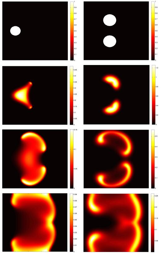
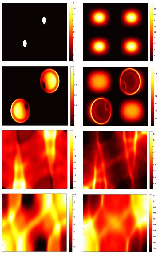
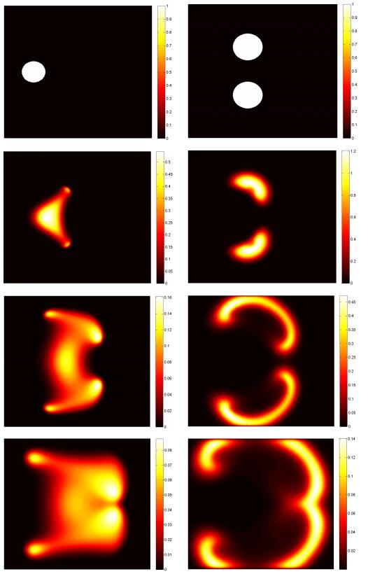
Reader Comments

Your name:*

Email:*
© 2019 the Author(s), licensee AIMS Press. This is an open access article distributed under the terms of the Creative Commons Attribution License (http://creativecommons.org/licenses/by/4.0)

通讯作者: 陈斌, bchen63@163.com

1.
沈阳化工大学材料科学与工程学院沈阳 110142

Mathematical Biosciences and Engineering

4.4

Metrics

Article views(6499) PDF downloads(1016) Cited by(21)

Preview PDF

Download XML

Export Citation

Article outline

Show full outline

Mathematical Biosciences and Engineering

A reaction-diffusion predator-prey model with pursuit, evasion, and nonlocal sensing

Related Papers:

Abstract

1. Introduction

2. Preliminary lemmas

3. Proof of theorem

3.1. Estimation of $R_{1}$

3.2. Estimation of $R_{2}$

4. Conclusions

Author contributions

Use of AI tools declaration

Acknowledgments

Conflict of interest

References

Reader Comments

通讯作者: 陈斌, bchen63@163.com

Metrics

Figures and Tables

Other Articles By Authors

Catalog

Abstract

1. Introduction

2. Preliminary lemmas

3. Proof of theorem

3.1. Estimation of $R_{1}$

3.2. Estimation of $R_{2}$

4. Conclusions

Author contributions

Use of AI tools declaration

Acknowledgments

Conflict of interest

References

Mathematical Biosciences and Engineering

A reaction-diffusion predator-prey model with pursuit, evasion, and nonlocal sensing

Related Papers:

Abstract

1. Introduction

2. Preliminary lemmas

3. Proof of theorem

3.1. Estimation of R1 R_{1}

3.2. Estimation of R2 R_{2}

4. Conclusions

Author contributions

Use of AI tools declaration

Acknowledgments

Conflict of interest

References

Reader Comments

通讯作者: 陈斌, bchen63@163.com

Metrics

Figures and Tables

Other Articles By Authors

Related pages

Tools

Export File

Citation

Format

Content

Catalog

Abstract

1. Introduction

2. Preliminary lemmas

3. Proof of theorem

3.1. Estimation of R_{1} R_{1}

3.2. Estimation of R_{2} R_{2}

4. Conclusions

Author contributions

Use of AI tools declaration

Acknowledgments

Conflict of interest

References

3.1. Estimation of $R_{1}$

3.2. Estimation of $R_{2}$

3.1. Estimation of $R_{1}$

3.2. Estimation of $R_{2}$