Research article Special Issues

Analysis of spontaneous emergence of cell polarity with delayed negative feedback

  • Cell polarity refers to spatial di erences in the shape and structure of cells, which leads to the generation of diverse cell types playing di erent roles in biological processes. Cell polarization usually involves the localization of some specific signaling molecules to a proper location of the cell membrane. Recent studies proposed that delayed negative feedback may be important for maintaining the robustness of cell polarization and the observed oscillating behavior of signaling cluster. However, the fundamental mechanisms for achieving cell polarization under negative feedback remain controversial. In this paper, we formulate the cell polarization system as a non-local reaction di usion equation with positive and delayed negative feedback loops. Through the Turing stability analysis, we identify the parameter conditions, including the range of the time delay constant, for achieving cell polarization without any inhomogeneous spatial cues. Also, our numerical results support that by controlling the length of the time delay in negative feedback and the magnitude of positive feedback, the oscillating behavior of signaling cluster can be observed in our simulations.

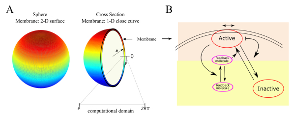
    Citation: Yue Liu, Wing-Cheong Lo. Analysis of spontaneous emergence of cell polarity with delayed negative feedback[J]. Mathematical Biosciences and Engineering, 2019, 16(3): 1392-1413. doi: 10.3934/mbe.2019068

    Related Papers:

    [1] Zhenzhen Zheng, Ching-Shan Chou, Tau-Mu Yi, Qing Nie . Mathematical analysis of steady-state solutions in compartment and continuum models of cell polarization. Mathematical Biosciences and Engineering, 2011, 8(4): 1135-1168. doi: 10.3934/mbe.2011.8.1135
    [2] Yuan Ma, Yunxian Dai . Stability and Hopf bifurcation analysis of a fractional-order ring-hub structure neural network with delays under parameters delay feedback control. Mathematical Biosciences and Engineering, 2023, 20(11): 20093-20115. doi: 10.3934/mbe.2023890
    [3] Ramesh Garimella, Uma Garimella, Weijiu Liu . A theoretic control approach in signal-controlled metabolic pathways. Mathematical Biosciences and Engineering, 2007, 4(3): 471-488. doi: 10.3934/mbe.2007.4.471
    [4] Juenu Yang, Fang Yan, Haihong Liu . Dynamic behavior of the p53-Mdm2 core module under the action of drug Nutlin and dual delays. Mathematical Biosciences and Engineering, 2021, 18(4): 3448-3468. doi: 10.3934/mbe.2021173
    [5] Gonzalo Robledo . Feedback stabilization for a chemostat with delayed output. Mathematical Biosciences and Engineering, 2009, 6(3): 629-647. doi: 10.3934/mbe.2009.6.629
    [6] Rongjian Lv, Hua Li, Qiubai Sun, Bowen Li . Model of strategy control for delayed panic spread in emergencies. Mathematical Biosciences and Engineering, 2024, 21(1): 75-95. doi: 10.3934/mbe.2024004
    [7] Jinhu Xu, Yicang Zhou . Bifurcation analysis of HIV-1 infection model with cell-to-cell transmission and immune response delay. Mathematical Biosciences and Engineering, 2016, 13(2): 343-367. doi: 10.3934/mbe.2015006
    [8] Anne C. Skeldon, Ian Purvey . The Effect of Different Forms for the Delay in A Model of the Nephron. Mathematical Biosciences and Engineering, 2005, 2(1): 97-109. doi: 10.3934/mbe.2005.2.97
    [9] Maria Vittoria Barbarossa, Christina Kuttler, Jonathan Zinsl . Delay equations modeling the effects of phase-specific drugs and immunotherapy on proliferating tumor cells. Mathematical Biosciences and Engineering, 2012, 9(2): 241-257. doi: 10.3934/mbe.2012.9.241
    [10] Lingli Zhou, Fengqing Fu, Yao Wang, Ling Yang . Interlocked feedback loops balance the adaptive immune response. Mathematical Biosciences and Engineering, 2022, 19(4): 4084-4100. doi: 10.3934/mbe.2022188
  • Cell polarity refers to spatial di erences in the shape and structure of cells, which leads to the generation of diverse cell types playing di erent roles in biological processes. Cell polarization usually involves the localization of some specific signaling molecules to a proper location of the cell membrane. Recent studies proposed that delayed negative feedback may be important for maintaining the robustness of cell polarization and the observed oscillating behavior of signaling cluster. However, the fundamental mechanisms for achieving cell polarization under negative feedback remain controversial. In this paper, we formulate the cell polarization system as a non-local reaction di usion equation with positive and delayed negative feedback loops. Through the Turing stability analysis, we identify the parameter conditions, including the range of the time delay constant, for achieving cell polarization without any inhomogeneous spatial cues. Also, our numerical results support that by controlling the length of the time delay in negative feedback and the magnitude of positive feedback, the oscillating behavior of signaling cluster can be observed in our simulations.


    Cell polarity refers to the asymmetric organization in the structure of cells and can enable cells to carry out specialized functions such as differentiation, migration and tissue development [1,2,3]. Disruption of cell polarity may lead to dysfunctionality of cells, which is usually a hallmark of human cancers [4,5]. Cell polarity always involves the localization of some specific signaling molecules to a proper location of the cell membrane [1,6], but the mechanism for achieving the localization remains controversial.

    The budding yeast Saccharomyces cerevisiae has been developed as an attractive model system to study cell polarization as its generation time is short and useful experimental tools are available in this system [1]. The axis of polarized growth is regulated by budding location at where a newborn cell emerges from the original cell. The polarization event of budding yeast involves a key polarity protein, Cdc42 GTPase, which is highly conserved from yeasts to humans and is critical in polarity establishment [7,8]. Cdc42 localizes at a site of polarized growth on the plasma membrane and interacts with several proteins to trigger downstream processes, resulting in the emergence and growth of a bud [1]. In a wild-type cell, the Cdc42 localization generally occurs in response to spatial cues that is dependent on cell type. However, yeast cells can still bud in the absence of spatial cues, but the bud site is selected at a fully random manner, so-called symmetry breaking [9,10]. A lot of previous experimental works have studied polarization in the absence of Rsr1, which connects the spatial cue and the downstream polarization pathway [9,11,12,13].

    Several mathematical models have been proposed to understand the mechanisms of achieving symmetry breaking in cell polarity [9,14,15,16,17]. More recently, in the geometric representation of a cell, studies [17,29] present bulk-surface reaction diffusion systems which incorporate cell membrane as surface and cytoplasm as bulk to investigate cell polarity in high dimensions. With the bulk-surface reaction diffusion models, classical linear stability analysis has been performed in literatures [17,30] and more recent approach, the local perturbation analysis, is also proposed [19,29]. Reaction-diffusion equation was always applied to model the budding process in yeast systems [14,15,16]. By the fact that the ratio of the diffusion rates of the cytoplasmic and membrane-bound Cdc42 is large, the Turing-type system became a possible mechanism for achieving symmetry breaking [14,16,18]. The key component of the Turing-type mechanism is the positive feedback loop in the cycle of Cdc42 and this concept was supported by a number of theoretical studies [14,16,17,18,19].

    Some experimental and theoretical studies indicated that negative feedback regulation exists during the formation of Cdc42 cluster [20,21,22,23,24]. Recent studies in [22,23,25] proposed that a delayed negative feedback may be important for maintaining the robustness of Cdc42 localization and the oscillating behavior of Cdc42 cluster during the process. However, cell polarization system with delayed negative feedback has not been studied with mathematical analysis in detail. In this paper, we first formulate a partial differential equation with positive and delayed negative feedback loops for studying cell polarization system. Then the Turing stability analysis is applied to identify the parameter conditions for achieving symmetry breaking during the process [14,26]. Our theoretical study provides us with several conditions for achieving a signaling cluster and simultaneously, these conditions include the constraint for the time delay in negative feedback loop. Numerical simulations are used to support our theoretical study and provide a full picture to understand the dynamics of cell polarization process. Also, our results support that the oscillating behavior of signaling cluster can be achieved by controlling the length of the time delay in negative feedback and the magnitude of positive feedback.

    This paper is organized as follows. In Section 2, we present a reaction-diffusion model of cell polarization with positive and delayed negative feedbacks. In Section 3, we perform the Turing stability analysis to the model proposed in Section 2 to derive the conditions for which cell polarity may emerge. Section 4 contains the studies of our numerical simulations. Finally, the conclusion is presented in Section 5.

    Here we consider a partial differential equation describing the dynamics of a polarized signaling molecule on the cell membrane (Figure 1). A recent study [29] of bulk-surface reaction diffusion models suggested that the geometry of the cell may affect the dynamics of polarized signaling molecules but here we assume that the cell is a sphere which is consistent with the situation of budding yeast. Under the assumption applied in [9,22], we consider that all cytoplasmic signaling molecules are inactive and all membrane-bound signaling molecules are active. The variable we consider here is the membrane-bound active form of the signaling molecules and the cytoplasmic inactive form of this molecule is modeled implicitly through the conservation of total molecules. This type of model was well applied to study Cdc42-GTPase cycle in budding yeast [9,22]. Most of the GTPase cycles have a common feature that enables them to switch between their active and inactive forms. The activation process is usually initiated by hydrolysis and can be reversed by Guanine nucleotide exchange factors (GEFs), which cause the GDP to dissociate from the GTP. For the membrane-bound form, GDIs release the GDP from the cell membrane to the cytoplasm through binding to the GTPase and it can also be reversed through the action of GDI displacement factors.

    Figure 1.  The spatial domains and feedback systems in the cell polarization model. A) Two-dimensional domain, represents the cell membrane, and simplified one-dimensional domain, represents the cross section of the cell membrane; B) System with a non-local positive feedback and delayed negative feedback. (): lateral diffusion; (): positive feedback; (): negative feedback; (): molecule transportation.

    The spatial domain in our model is the membrane of a cell of radius R μm denoted by M, which is a sphere (two-dimensional domain), or, for simplicity, we can only consider the cross section of the cell membrane, which is a circle (one-dimensional domain) (shown in Figure 1A). We use a variable a to represent the particle fractions of the membrane-bound active signaling molecules [9]. The dynamic of a is governed by a reaction-diffusion equation with the feedback functions F(,) and G():

    a(t,x)t=Dm2a(t,x)+F(a(t,x),^a2(t))(1ˆa(t))G(a(tτ,x))a(t,x), (2.1)

    with ˆa(t)=Ma(t,x) dSx/|M| and ^a2(t)=Ma2(t,x) dSx/|M|, respectively representing the average values of a and a2 over the cell membrane, and |M| equals to the total area of the domain M. The first term of the right-hand side represents the diffusion of signaling molecules with the lateral surface diffusion rate coefficient Dm and the Laplace operator 2 on the cell membrane.

    In our model, we assume that the total number of signaling molecules in the whole cell is conserved. With the fact that ˆa represents the total fractions of the membrane bound species, we obtain

    N=(ˆa+Fracc)N, (2.2)

    where Fracc is the fraction of cytoplasmic inactive signaling molecules and N is the total number of signaling molecules, including active and inactive forms, in the whole cell. Hence, by (2.2), Fracc=1ˆa. Due to the fast cytoplasmic diffusion, we assume that signaling molecules are uniformly distributed throughout the cytoplasm. By assuming the activation rate is proportional to the fraction of cytoplasmic signaling molecules, the term F(a,^a2)(1ˆa) in (2.1) is applied to model the activation process in the system.

    In budding yeast, there is a positive feedback loop to promote Cdc42 activation [9,22]. Here we assume that the activation rate is positively regulated by the active molecules a and thus the function F is an increasing function of a (Figure 1B). In this paper, we define the feedback function as

    F(a,^a2)=konk1+k2a21+k1+k2^a2. (2.3)

    This feedback function models multi-step cooperative interactions which has been used in several biological Turing type systems [26]. The nonlinear cooperativity is modeled by the term a2, the degree of cooperativity is 2 [22]. The function form in (2.3) depends on a non-local term ^a2 and the local density a. The feedback is mediated through a special type of molecules initially uniformly distributed in the cytoplasm, such as the Bem1 complex in the Cdc42 cycle of budding yeast [18,27]. The detailed derivation of this feedback function can be found in A.1.

    The observed oscillation and fluctuation of Cdc42 cluster support that the delayed negative feedback is involved in the cell polarization system of budding yeast [22]. We assume that the deactivation function G depends on the value of a(tτ,x) with a delay time of τ, as the deactivation rate varies with the activation level of Rga1, which may be regulated by the level of Cdc42 in budding yeast (Figure 1B). Here we apply a linear function to model the deactivation rate G in (2.1):

    G(a(tτ,x))=g1+g2a(tτ,x). (2.4)

    The studies in [11] show that the necessary condition for achieving Cdc42 localization is that the rate of activation grows faster with the increase in active Cdc42 than the rate of deactivation, so that the linear function is used here instead of higher order functions.

    In this section, the Turing stability analysis is applied to figure out the conditions of the parameters to achieve spontaneous cell polarization [26]. The analysis in this section can be applied for the system with general feedback functions F(a,^a2) and G(a(tτ,x)).

    For studying the stability of a homogeneous steady state solution, we first study a homogeneous steady state solution a0 of the system (2.1). Since a0 is homogeneous over space, ^a20=a20 and the solution a0 satisfies the following equation:

    0=F(a0,a20)(1a0)G(a0)a0. (3.1)

    Since F and G are positive functions, the right-hand side of (3.1) is negative when a0=1; the right-hand side of (3.1) is positive when a0=0. By the intermediate value theorem, at least one homogeneous positive steady state solution a0 exists between 0 and 1.

    Here we define a(t,x) as slightly perturbed functions from the homogeneous steady state a0:

    a(t,x)=a0+ϵa1(t,x), (3.2)

    where the perturbation amplitude ϵ1 is much smaller than the value of a0. After substituting (3.2) into Eq. (2.1) and applying Taylor expansion around a0, the leading terms satisfy the following system:

    a1t=Dm2a1+(FX1(a0,a20)a1+2a0^a1FX2(a0,a20))(1a0)G(a0)a1GX(a0)a0a1F(a0,a20)^a1, (3.3)

    where a1=a1(tτ,x); FX1 and FX2 denote the partial derivatives of F with respect to the first and the second arguments, respectively; GX denotes the first derivative of G. When the feedback functions (2.3) and (2.4) are considered, we obtain that FX1 is positive, FX2 is negative and GX is positive. A particular spatially periodic perturbation function, a1(t,x)=αeλtEw(x), is considered here. In the function, α is a nonzero parameters, w is a non-negative integer and Ew(x) is the w-th non-zero eigenfunction of the Laplace operator. Eq. (3.3) becomes

    λ=σwDm+(FX1+2a0FX2δ(w))(1a0)GGXa0eλτFδ(w), (3.4)

    where

    δ(w)={1if w=0,0if w>0,

    and the eigenvalue

    σw={w2/R2for the one-dimensional domain;2w2/R2for the two-dimensional domain,

    where R is the radius of the circle; FX1,FX2,F,G,GX are evaluated at (a0,a20).

    The emergence of cell polarity usually depends on the instability of the homogeneous steady state, which requires two conditions [16,26]:

    (1) If the perturbation is spatially homogeneous (w=0), the homogeneous steady state a0 is linearly stable. This condition is equivalent to that the real parts of all eigenvalues λ are negative when the wave number w is zero. This condition ensures that a homogeneous solution starting from a constant initial condition close to a0 will finally tend to a0.

    (2) The homogeneous steady state a0 is linearly unstable under a perturbation with a positive wave number w. This condition is equivalent to that there exists a positive integer w such that at least one λ satisfying (3.4) has a positive real part.

    These two conditions imply that the random perturbed homogeneous steady state are moving toward another inhomogeneous steady state for and only for positive wave lengths.

    Eq. (3.4) has a form

    λ=Aw+Beλτ, (3.5)

    where

    Aw=σwDm+(FX1+2a0FX2δ(w))(1a0)GFδ(w)

    and

    B=GXa0.

    According to [28], we can determine the signs of all possible λ by the following theorem:

    Theorem 1 (Theorem 4.7 from [28]). For Eq. (3.5), we have

    (a) If Aw+B>0, then there exists at least one λ with positive real part;

    (b) If Aw+B<0 and AwB0, then all λ have negative real parts;

    (c) If Aw+B<0 and AwB>0, then there exists

    τ=(B2A2w)1/2cos1(Aw/B)>0

    such that (1) all λ have negative real parts for 0<τ<τ, and (2) there exists at least one λ with positive real part for τ>τ.

    Condition (1)

    By Theorem 1, the condition (1) is equivalent to that when w=0, we have

    Theorem 1(b):A0+B<0 and A0B0;

    or

    Theorem 1(c):A0+B<0A0B
     and 0τ<(B2A20)1/2cos1(A0/B),

    where A0=(FX1+2a0FX2)(1a0)GF and B=GXa0.

    Since B is always negative, we have A0B>A0+B and |B|=B so

    A0B0 implies A0+B<0

    and

    A0+B<0 and A0B>0 if and only if |A0|<|B|.

    So the two situations for satisfying the condition (1) can be simplified as the following two cases:

    Case (1a):A0B0

    or

    Case (1b):|A0|<|B| and 0τ<(B2A20)1/2cos1(A0/B).

    From Cases (1a) and (1b), we can see that if the time delay τ is large and A0B>0, the homogeneous steady state is not stable for a homogeneous perturbation. Under this situation, the steady state does not satisfy the condition (1) of Turing instability. For studying this situation, we consider the spatial homogeneous system from the model (2.1):

    dˉadt=konk1+k2ˉa21+k1+k2ˉa2(1ˉa)(g1+g2ˉa(tτ))ˉa.

    It is easy to show that the solution ˉa is bounded between 0 and 1 with ˉa(0)(0,1). If all steady states of ˉa are not stable for a large time delay τ, the solution is under oscillation around some homogeneous steady states. Hence, for the original system (2.1), the instability for some positive wave number w>0 may still contribute to achieve inhomogeneous pattern when the condition (2) is satisfied and the solution is close to the homogeneous steady state. Our simulation results shown in the later section will demonstrate that, with a large time delay, a cluster of signaling molecules can be formed from a homogeneous steady state with a small inhomogeneous perturbation even though all homogeneous steady state is not stable for w=0.

    Condition (2) By Theorem 1, the condition (2) is equivalent to the situation that for some positive integers w>0, we have

    Theorem 1(a):Aw+B>0;

    or

    Theorem 1(c):Aw+B<0,AwB>0 and τ>(B2A2w)1/2cos1(Aw/B),

    where Aw=σwDm+FX1(1a0)G and B is defined above.

    Since Aw is decreasing with respect to w for w1, the two cases can be simplified to the situation only for w=1:

    Case (2a):A1+B>0

    or

    Case (2b):|A1|<|B| and τ>(B2A21)1/2cos1(A1/B).

    where A1=σ1Dm+FX1(1a0)G.

    To obtain Turing instability, at least one of Cases (2a) and (2b) has to be satisfied. The following two propositions provide the necessary conditions for obtaining at least one of Cases (2a) and (2b).

    Proposition 2. For the system (2.1) with the feedback forms (2.3) and (2.4), Case (2a) is satisfied only if

    konk2>g2. (3.6)

    Proof. Case (2a) can be written as

    A1+B=kon2k2a01+k1+k2a20(1a0)(g1+2g2a0)σ1Dm>0. (3.7)

    Since

    kon2k2a01+k1+k2a20(1a0)(g1+2g2a0)σ1Dm<2(konk2g2)a0,

    Case (2a) implies konk2>g2.

    Proposition 3. For the system (2.1) with the feedback forms (2.3) and (2.4), Case (2a) or Case (2b) is satisfied only if

    konk2>12(g1+σ1Dm). (3.8)

    Proof. If Case (2a) or Case (2b) is true, we have A1B>0 which can be written as

    A1B=kon2k2a01+k1+k2a20(1a0)g1σ1Dm>0. (3.9)

    Since

    kon2k2a01+k1+k2a20(1a0)g1σ1Dm<2konk2g1σ1Dm,

    the inequality (3.9) implies konk2>12(g1+σ1Dm).

    The two propositions show that konk2 has to be large enough for achieving Turing instability. Other than the necessary conditions, the following theorem provides a sufficient condition for determining a range of parameters in which Case (2a) is satisfied:

    Theorem 4. Assume that σ1Dm<konk1. For the system (2.1) with the feedback forms (2.3) and (2.4), Case (2a) is satisfied if

    112kon(g2k2+g22k22+(g1+σ1Dm)2k1k2)>0 (3.10)

    and

    k1g2k2+k21g22k22+(g1+σ1Dm)2k1k2<(g1σ1Dm)[(kon+g1)24g22+kong2(112kon(g2k2+g22k22+(g1+σ1Dm)2k1k2))kon+g12g2]. (3.11)

    The proof of Theorem 4 is based on the method used in [14] and the detailed proof is presented in A.2. It is worth noting that the necessary and sufficient conditions can be obtained by the formula for the roots of quadratic equation but the formula is too complicated and not applicable for parameter estimation.

    The conditions obtained in Theorem 4 provide a good insight on the range of parameters for achieving Case (2a). For example, Theorem 4 implies that there exist a constant k>0 such that Case (2a) is satisfied if kon>k. Figure 2 displays the numerical results for determining how close between the conditions in Theorem 4 and the exact range for achieving Case (2a). In the figure, we consider 1000 sets of different (k2,g2) generated uniformly within [1,100]×[1,10], and choose the remaining parameters within the ranges: σ1Dm=[0.025,0.225]/min, kon[1,5]/min, k1=1, g1=1/min, which are based on some previous works [22,27].

    Figure 2.  The stability diagrams for the system (2.1) with the feedback forms (2.3) and (2.4) with different kon and σ1Dm. A) The ranges of the parameters that satisfy the conditions provided in Theorem 4. Brown region represents the ranges that satisfy the conditions; Green region represents the ranges that do not satisfy the conditions. B) The ranges of the parameters that satisfy Case (2a). Brown region represents the ranges that satisfy Case (2a); Green region represents the ranges that do not satisfy Case (2a). C) The difference between the ranges obtained in (A) and (B). Brown region represents the ranges that the results in (A) and (B) are not consistent; Green region represents the ranges that the results in (A) and (B) are consistent.

    Although the conditions in Theorem 4 (the brown regions in Figure 2A) are just sufficient conditions for Case (2a), they still have a good agreement with the exact range for Case (2a) (the brown regions in Figure 2B) and the difference appears only in a few sets of parameters (Figure 2C). The numerical results in Figure 2 show that the difference between the conditions in Theorem 4 and the exact region for Case (2a) can be minimized by reducing the membrane-bound diffusion coefficient Dm which is usually small (<0.5μm2/min) in budding yeast system [22,27].

    Linear stability analysis only focuses on the local behavior near the homogeneous steady state. Here we apply numerical simulations to study the long-term behavior of the system under different stability conditions studied in the previous section.

    First, we use a computational simulation for one-dimensional model to study the ranges of the parameters for satisfying the two stability conditions (1) and (2). 10,000 sets of different (k2,g2) are uniformly generated within the region [1,100]×[1,100]. Other parameters are set as follows: Dm=0.1μm2/min, kon[1,5]/min, k1=1, g1=1/min, τ[0.1,1]min. Here Dm was obtained by the smallest value of σ1Dm (σ1Dm=0.025/min and σ1=1/R2) in Figure 2 which has given the conclusion that smaller Dm can reduce the difference between conditions in Theorem 4 and the exact region for Case (2a). Figure 3 displays the stability diagrams for kon=1/min,3/min and 5/min and τ=0.1min,0.5min and 1min. Figure 3A shows the ranges of the parameters that satisfy the condition (1) (the stability condition for homogeneous perturbation with w=0); Figure 3B shows the ranges of the parameters that satisfy the condition (2) (the stability condition for inhomogeneous perturbation with w=1).

    Figure 3.  The stability diagrams for the system (2.1) with the feedback forms (2.3) and (2.4) with different kon values and τ values. A) The ranges of parameters that satisfy the condition (1). B) The ranges of parameters that satisfy the condition (2). Brown region represents the ranges that satisfy the condition; Green region represents the ranges that do not satisfy the condition.

    According to the results in Figure 3, different combinations of parameters are chosen under different stability conditions. Here we fix the parameters Dm=0.1μm2/min, kon=3/min, k1=1 and g1=1/min [22,27]. For other parameters, we choose within the ranges k2[1,100], g2[1,100]/min and τ[0.1,1]min. Under this parameter setting, the system has a unique homogeneous steady state solution a0. In all the simulations throughout this paper, the initial conditions are the homogeneous steady states with spatial perturbation (±10% perturbation):

    a(t,x)=a0(1+0.1η(x)), for τt0,

    where η(x) is a function of uniformly distributed random number between -1 and 1. If the perturbation is large, the initial condition may be larger than 1. Within the ranges of the parameters we tested, we have verified that 1.1a0<1. In some cases, larger perturbation (±20%) is also considered for further study and the results are consistent with what we observed here. We apply the second-order central difference approximation for the diffusion term, periodic boundary conditions for two end sides, Riemann sum for the definite integrals and the built-in function dde23 in the MATLAB for the temporal simulation with the constant time delay τ. For the spatial discretization, the number of spatial points is 300 with uniform distribution and the radius of the circle is R=2μm.

    Figure 4 demonstrates the simulations for g2=5/min which represents the cases that the magnitude of negative feedback is low. When τ=0.1min (short time delay) and k2=20 (weak positive feedback), the system does not satisfy the condition (2) and the numerical simulation in Figure 4A shows that the concentration of a rapidly returns back to the homogeneous steady state. When the magnitude of positive feedback (k2) increases to 50 or higher, the system satisfies the two conditions (1) and (2) and inhomogeneous patterns can be always observed in the simulation (Figure 4A). Figure 4B shows that when τ is increased to be 0.5min, a cluster of signaling molecules does not exist if the condition (2) is not satisfied, such as k2=20 (weak positive feedback). When k2 increases to 50 or higher, a cluster of signaling molecules appears but is not stable at a certain location. In this case, the signaling cluster is traveling with constant speed and keeps moving until the end.

    Figure 4.  The simulations for the one-dimensional model with weak negative feedback, g2=5/min. In the simulations, we set Dm=0.1μm2/min, kon=3/min, k1=1, g1=1/min, k2[20,100], τ=0.1min (in A), 0.5min (in B). The horizontal axis represents time evolution and the vertical axis represents membrane position (shown in the left panel).

    For stronger negative feedback (g2=50/min or 100/min) with large enough time delay and positive feedback, a cluster of signaling molecules can appear but may not be stable at a certain location. Figure 5A demonstrates that when τ=0.1min and the system does not satisfy the condition (2), the concentration of a rapidly returns back to the homogeneous steady state even under a strong positive feedback.

    Figure 5.  The simulations for the one-dimensional model with strong negative feedback, g2=50/min (in A-C) and g2=100/min (in D). In the simulations, we set Dm=0.1μm2/min, kon=3/min, k1=1, g1=1/min, k2[15,100], τ=0.1min (in A), 0.5min (in B), 1min (in C-D). The horizontal axis represents time evolution and the vertical axis represents membrane position (as in Figure 4).

    Figures 5B-D show that how the dynamics of the signaling clusters change when the magnitude of the positive feedback increases from 5 to 50. Interestingly, when k215, Case (2b) is satisfied and an inhomogeneous pattern is observed: for k2=15, the concentration of a signaling cluster is oscillating during the process; when k2 increases to 50, a traveling signaling cluster appears. In Figure 5D, when k2=50, both Case (1a) and Case (1b) are not satisfied so the homogeneous steady state is unstable for a homogeneous perturbation w=0. The simulation shows that a signaling cluster can be obtained in this case even though the homogeneous steady state is not stable when w=0. But this situation is usually with larger time delay constant so the signaling cluster may not be stable at a certain location.

    Figure 6 summarizes the simulation results for studying how the long-term behavior of the system depends on the values of k2 and τ with two different levels of negative feedback, g2=5/min,50/min. The results are consistent with our previous stability analysis. From this result, we observe that suitable ranges of the magnitude of positive feedback and time delay are important for achieving an oscillation of signaling cluster, observed in experiments [22]. It is worth noting that although the numerical results obtained here only focused on a simplified domain (the one-dimensional domain for the cross section of the cell), we can apply the results onto the the two-dimensional spherical surface. Figure 7 displays three examples of the simulations on the two-dimensional spherical surface. For the spatial discretization, the number of spatial points is 4098 with uniform distribution and the radius of the circle is R=2μm. These three simulations are corresponding to the one-dimensional simulations shown in Fig 4A and Figures 5B and C. In Figure 7A, a stable cluster is formed until the end; in Figures 7B, C, the concentration of the signaling cluster is oscillating during the process. The results in these three cases are consistent with what observed in the one-dimensional simulations.

    Figure 6.  The long-term behavior of the system with different values of k2, τ and g2. A) Weak negative feedback, g2=5/min. Blue region: no cluster is formed; green region: a traveling signaling cluster is observed; yellow region: a stable signaling cluster is formed. B) Strong negative feedback, g2=50/min. For the simulations, 100 sets of different (k2,τ) are uniformly generated within the region [1,50]×[0.1,0.5]. Blue region: no cluster is formed; green region: a traveling signaling cluster is observed; yellow region: an oscillating cluster is observed.
    Figure 7.  Time-dependent solutions of a for the two-dimensional model. In the simulations, Dm=0.1μm2/min; kon=3/min; k1=1; k2=50 (in A), 15 (in B, C); g1=1/min; g2=5/min (in A), 50/min (in B, C); τ=0.1min (in A), 0.5min (in B), 1min (in C).

    Recent experimental studies demonstrated that delayed negative feedback regulation may play an important role in robustness of Cdc42 localization and the oscillating behavior of Cdc42 cluster during cell polarization [22]. However, detailed mathematical analysis is not well studied for this system.

    In this paper, we have built a simple model of reaction-diffusion equation for cell polarization system which is regulated by positive and delayed negative feedback together. Our model involves general forms of positive and negative feedbacks. We have applied Turing stability analysis to analyze the conditions that can give rise to spontaneous cell polarization. Moreover, our numerical studies reveal that Cdc42 cluster can form but may not be spatially stable when the time delay τ is large. Also, our numerical results support that the oscillating behavior of Cdc42 cluster can be achieved by controlling the length of time delay and the magnitude of positive feedback.

    The results in this paper provide parameter conditions for the existence of polarized solutions in the cell polarization system with delayed negative feedback. Furthermore, the analysis of the feedback can be easily extended to higher dimensional domain and provides insights to understand other similar biological systems in which cell polarity is established. Also, like the study in [22], our results can be used to study how the spatial cue level and the time delay affect the oscillating behavior by involving a spatial cue function kcue in the positive feedback term:

    F(x,a,^a2)=kcue(x)+konk1+k2a21+k1+k2^a2, (5.1)

    where

    kcue(x)={C0if x[π0.25,π+0.25],0otherwise.

    In the future work, our model can be combined with a moving boundary system for cell shape change during budding, then we can extend our study of Cdc42 localization to cell morphogenesis.

    WCL was partially supported by a CityU Strategic Research Grant (Project No. 7004697) and a grant from the Research Grants Council of the Hong Kong Special Administrative Region, China (Project No. CityU 11303117).

    All authors declare no conflicts of interest in this paper.

    We assume that the feedback molecules, as shown in Figure 1B, are initially uniformly distributed in the cytoplasm and then the active signaling molecules will recruit them to the cell membrane. On the other hand, the activation rate of the signaling molecules is proportional to the density of the membrane-bound feedback molecules. Therefore, we obtain the following equation for c:

    ct=(h1+h2a2)(1ˆc)hoffc, (A.1)

    where (h1+h2a2) and hoff are the recruitment rate and the dissociation rate of the feedback molecules, respectively; (1ˆc) is the fraction of the cytoplasmic feedback molecules (ˆc is the average value of c over the membrane).

    We know that the dynamics of the feedback molecules is much faster than that of the signaling molecules [18,27], the variable c can be approximated by the solution of the quasi steady state equation of Eq. (A.1):

    (h1+h2an)(1ˆc)hoffc=0.

    By integrating the above equation over the membrane, we can obtain the value of ˆc. After substituting ˆc back into the equation, we have

    c=k1+k2an1+k1+k2^an,

    where k1 and k2 equal to h1/hoff and h2/hoff, respectively. We assume that the feedback strength is linearly proportional to the value of c, then we obtain the feedback function (2.3).

    Here we will state two lemmas, which will be used in Section A.2.2 for the proofs of Theorems 4. First, we define a function fy(a) used in the lemmas:

    fy(a)=(γ1+γ2a2)(1γ3yγ4y2)γ5aγ6a2D(ay). (A.2)

    where γ1,γ2,γ4,γ5,γ6>0, γ31 and 0D<γ1γ3.

    Lemma 5. Assume that γ2>γ6 and y[0,y] where γ2(1γ3yγ4y2)γ6=0. The function fy in (A.2) has the following properties:

    1. mina0fy(a) equals to

    γ1(γ1γ3D)yγ1γ4y2(γ5+D)24(γ2(1γ3yγ4y2)γ6),

    which is strictly decreasing with respect to y for y(0,y).

    2. For each y, there exist at most two solutions in {a|a0} satisfying fy(a)=0.

    3. There exists a number ym in [0,y) such that two smooth functions a1(y), a2(y) can be well defined in the domain [ym,y) and the following properties hold:

    (a) mina0fy(a)0 for any y[ym,y);

    (b) fy(a1(y))=fy(a2(y))=0 for any y[ym,y);

    (c) a1(y)>a2(y)0 for any y(ym,y);

    (d) a1(y)>0 and a2(y)<0 for any y(ym,y);

    (e) limyya1(y)= and limyya2(y)=0;

    (f) dfyda|a=a1(y)>0 and dfyda|a=a2(y)<0 for any y(ym,</italic><italic>y);

    (g) if there is at least one solution in a0 for f0(a)=0, then ym=0;

    (h) if there is no solution in a0 for f0(a)=0, then a1(ym)=a2(ym), dfymda|a=a1(ym)=dfymda|a=a2(ym)=0 and mina0fym(a)=0.

    Proof. 1. First we consider the first and second derivatives of fy,

    dfy(a)da=2γ2a(1γ3yγ4y2)γ52γ6aD, (A.3)
    d2fy(a)da2=2γ2(1γ3yγ4y2)2γ6. (A.4)

    By Eq. (A.4), we show that d2fy(a)da2>0 for y[0,y) and the minimum point in {a|a0} is at

    a=γ5+D2γ2(1γ3yγ4y2)2γ6

    with

    mina0fy(a)=γ1(γ1γ3D)yγ1γ4y2(γ5+D)24(γ2(1γ3yγ4y2)γ6).

    By the given condition D<γ1γ3, we can show that mina0fy(a) is strictly decreasing with respect to y.

    2. Suppose that y is a fixed number. If mina0fy(a)>0, there is no solution a0 satisfying fy(a)=0.

    If mina0fy(a)=0, the minimum point

    ˉa=γ5+D2γ2(1γ3yγ4y2)2γ6

    is one of the roots for fy(a). As dfy(a)da>0 for a>ˉa and dfy(a)da<0 for 0a<ˉa, fy(a)>fy(ˉa) for any aˉa, and therefore ˉa is the only solution of fy(a)=0.

    If mina0fy(a)<0, by the fact that fy(0)>0, limafy(a)>0 and the intermediate value theorem, we can show that there are at least two solutions satisfying fy(a)=0. As dfy(a)da>0 for a>ˉa and dfy(a)da<0 for 0a<ˉa, fy(a)>fy(ˉa) for any aˉa. So there are only two roots of fy(a): one is in [0,ˉa), and the other is in (ˉa,).

    3. By the result of part 1, mina0fy(a) tends to as y is close to y. If mina0fy(a)>0 for y=0, according to the intermediate value theorem, we can find ym such that mina0fym(a) equals zero; if mina0fy(a)0 for y=0, we define ym=0.

    Since mina0fy(a) is strictly decreasing with respect to y, and according to the results of part 2, fy(a)=0 has two solutions a for any y(ym,y), so we can define two functions a1(y) and a2(y) that satisfy fy(a1(y))=fy(a2(y))=0 and a1(y)>a2(y) for any y(ym,y), that is,

    a1(y)=max{a0|fy(a)=0},a2(y)=min{a0|fy(a)=0}.

    The derivative of fy(a) with respect to y is (γ1+γ2a2)(γ3+2γ4y)+D, which is always negative due to γ1γ3>D, and fy(a) is a smooth function with respect to y and a, and therefore we can apply the inverse function theorem to show that a1(y) and a2(y) are smooth functions. By the definitions and the proof of part 2, it is easy to verify the properties (a, b, c, f, g, h).

    By property (b), we have fy(a1(y))=0 and fy(a2(y))=0. By differentiating these two equations with respect to y on both sides, we have (γ1+γ2a1(y)2)(γ3+2γ4y)+D+dfyda(a1(y))a1(y)=0 and (γ1+γ2a2(y)2)(γ3+2γ4y)+D+dfyda(a2(y))a2(y)=0. Hence we obtain

    a1(y)=(γ1+γ2a1(y)2)(γ3+2γ4y)+Ddfyda(a1(y)),a2(y)=(γ1+γ2a2(y)2)(γ3+2γ4y)+Ddfyda(a2(y)).

    By property (f) and γ1γ3>D, we proved that a1(y)>0 and a2(y)<0, which completes the proof of property (d).

    From the proof of part 2, we have a2[0,ˉa) and a1(ˉa,). So we know that a1(y) tends to infinity as y goes to y. Since a=0 is the solution for fy(a)=0, we have limyya2(y)=0, which completes the proof of property (e).

    Lemma 6. Let Ω be a solution of

    (γ5+D)24(γ2(1γ3Ωγ4Ω2)γ6)+γ1(1γ3Ωγ4Ω2)=0, (A.5)

    and assume that Ω>0 and γ2>γ6. If

    2γ1(1γ3Ωγ4Ω2)+(Dγ5)Ω<0 (A.6)

    is satisfied, then dfa0da|a=a0>0 holds for any solution a0 satisfying fa0(a0)=0.

    For the proofs of Lemmas 6, we define two functions S1, S2 in the domain [ym,1/γ3):

    S1(y)=a1(y)y,S2(y)=a2(y)y,

    where a1, a2 and ym are defined in Lemma 5.

    Proof. There are two parts in the proof:

    1. Prove that if S1(ym)<0, dfa0da|a=a0>0 holds for any solution a00 satisfying fa0(a0)=0.

    2. Prove that condition (A.6) implies S1(ym)<0.

    By combining these two results, we can prove that if the condition (A.6) is satisfied, then dfa0da|a=a0>0 holds for any solution a00 satisfying fa0(a0)=0.

    Proof of part 1: Suppose that S1(ym)<0. Since a1(y)a2(y), we get S2(ym)S1(ym)<0. By a2(y)<0 (Lemma 5(3c)), we have S2<0, which means that S2 is a decreasing function. Since S2(ym)<0 and S2 is a decreasing function, S2(y)<0 for all y[ym,y), and there is no solution to S2(y)=0.

    According to Lemma 5 and the definitions of S1 and S2, all solutions a00 for fa0(a0)=0 have to satisfy S1(a0)=0 or S2(a0)=0. Since S1(ym)<0 implies that there is no solution satisfying S2(y)=0, all solutions a00 for fa0(a0) have to satisfy S1(a0)=0 and therefore dfa0da|a=a0>0 according to Lemma 5(3f).

    Proof of part 2: Suppose that condition (A.6) is satisfied, by Lemma 5(1), we have

    mina0fy(a)=γ1(γ1γ3D)yγ1γ4y2(γ5+D)24(γ2(1γ3yγ4y2)γ6).

    If 0<y<Ω, we have

    (γ5+D)24(γ2(1γ3yγ4y2)γ6)+γ1(1γ3yγ4y2)>0(γ5+D)24(γ2(1γ3yγ4y2)γ6)+γ1(1γ3yγ4y2)+Dy>0mina0fy(a)>0. (A.7)

    Lemma 5(3a) implies that mina0fym(a)>0 so ym is larger than Ω>0. Then we apply Lemma 5(3h) to show that there is no solution with a0 such that f0(a)=0.

    By Lemma 5(3b, h), we know that (ym,a1(ym)) satisfies the following two equations:

    fym(am)=(γ1+γ2a2m)(1γ3ymγ4y2m)γ5amγ6a2mD(amym)=0, (A.8)
    dfymda|a=am=2γ2am(1γ3ymγ4y2m)γ52γ6amD=0, (A.9)

    where am=a1(ym).

    After multiplying (A.8) and (A.9) by n and am, respectively, we have

    2(γ1+γ2a2m)(1γ3ymy4y2m)2γ5am2γ6a2m2D(amym)=0, (A.10)
    2γ2a2m(1γ3ymγ4y2m)γ5am2γ6a2mDam=0. (A.11)

    Subtracting (A.10) by (A.11), we obtain

    2γ1(1γ3ymγ4y2m)γ5am+2DymDam=0,

    which leads to

    am=2γ5+D(γ1(1γ3ymγ4y2m)+Dym). (A.12)

    By substituting (A.12) into S1(ym), we obtain

    S1(ym)=amym=1γ5+D(2γ1(1γ3ymγ4y2m)+(Dγ5)ym). (A.13)

    By applying ym>Ω>0, D<γ1γ3 and condition (A.6),

    2γ1(1γ3ymγ4y2m)+(Dγ5)ym<0

    which, coupled with (A.13), implies that S1(ym)<0.

    Proof. First, we set γ1=konk1, γ2=konk2, γ3=kon+g1kon>1, γ4=g2kon, γ5=g1, γ6=g2 and D=σ1Dm used in the lemmas.

    Solving (A.5) in Lemma 6, we obtain

    Ω=((kon+g1)24g22+kong2(112kon(g2k2+g22k22+(g1+σ1Dm)2k1k2))kon+g12g2)

    By the condition (3.10) of Theorem 4

    112kon(g2k2+g22k22+(g1+σ1Dm)2k1k2)>0

    we have Ω>0 and γ2=konk2>γ6=g2. Also the other condition (3.11) of Theorem 4

    k1g2k2+k21g22k22+(g1+σ1Dm)2k1k2<(g1σ1Dm)((kon+g1)24g22+kong2(112kon(g2k2+g22k22+(g1+σ1Dm)2k1k2))kon+g12g2)

    implies the condition (A.6). By Lemma 6, we have

    2konk2a0(1kon+g1kona0g2kona20)(g1+2g2a0)σ1Dm>0 (A.14)

    holds for any a0 satisfying

    kon(k1+k2a20)(1kon+g1kona0g2kona20)(g1+g2a0)a0=0. (A.15)

    Eq. (A.15) implies that

    kon(k1+k2a20)(1a0)(1+k1+k2a20)(g1+g2a0)a0=0konk1+k2a201+k1+k2a20(1a0)(g1+g2a0)a0=0 (A.16)

    Now we get that a0 is a homogeneous steady state solution for a in system (2.1) with the feedback forms (2.3) and (2.4) if and only if a0 satisfies (A.15).

    Also, (A.16) and (A.15) imply that

    11+k1+k2a20(1a0)=1kon+g1kona0g2kona20

    and then combining (A.14), we have

    kon2k2a01+k1+k2a20(1a0)(g1+2g2a0)σ1Dm>0

    which is equivalent to Case (2a).


    [1] E. Bi and H. O. Park, Cell polarization and cytokinesis in budding yeast, Genetics, 191 (2012), 347–387.
    [2] D. M. Bryant and K. E. Mostov, From cells to organs: building polarized tissue, Nat. Rev. Mol. Cell Biol., 9 (2008), 887–901.
    [3] D. G. Drubin and W. J. Nelson, Origins of cell polarity, Cell, 84 (1996), 335–344.
    [4] M. E. Lee and V. Vasioukhin, Cell polarity and cancer–cell and tissue polarity as a non-canonical tumor suppressor, J. Cell Sci., 121 (2018), 1141–1150.
    [5] C. Royer and X. Lu, Epithelial cell polarity: a major gatekeeper against cancer?, Cell Death. Differ., 18 (2011), 1470–1477.
    [6] H. O. Park and E. Bi, Microbiology and Molecular Biology Reviews, Microbiol. Mol. Biol. Rev., 71 (2007), 48–96.
    [7] H. R. Bourne, D. A. Sanders and F. McCormick, The GTPase superfamily: a conserved switch for diverse cell functions, Nature, 348 (1990), 125–132.
    [8] S. Etienne-Manneville and A. Hall, Rho GTPases in cell biology, Nature, 420 (2002), 629–635.
    [9] S. J. Altschuler, S. B. Angenent, Y. Wang and L. F. Wang, On the spontaneous emergence of cell polarity, Nature, 454 (2008), 886–889.
    [10] B. D. Slaughter, S. E. Smith and R. Li, Symmetry breaking in the life cycle of the budding yeast, Csh. Perspect. Biol., 1 (2009), a003384.
    [11] A. B. Goryachev and M. Leda, Many roads to symmetry breaking: molecular mechanisms and theoretical models of yeast cell polarity, Mol. Biol. Cell, 28 (2017), 370–380.
    [12] J. M. Johnson, M. Jin and D. J. Lew, Symmetry breaking and the establishment of cell polarity in budding yeast, Curr. Opin. Genet. Dev., 21 (2011), 740–746.
    [13] S. G. Martin, Spontaneous cell polarization: Feedback control of Cdc42 GTPase breaks cellular symmetry, BioEssays, 37 (2015), 1193–1201.
    [14] W. C. Lo, H. O. Park and C.S. Chou, Mathematical analysis of spontaneous emergence of cell Polarity, Bull. Math. Biol., 76 (2014), 1835–1865.
    [15] Y. Mori, A. Jilkine and L. Edelstein-Keshet, Wave-pinning and cell polarity from a bistable reaction-diffusion system, Biophys J., 94 (2008), 3684–3697.
    [16] A. Rätz and M. Röger, Turing instabilities in a mathematical model for signaling networks, J. Math. Biol., 65 (2012), 1215–1244.
    [17] A. Rätz and M. Röger, Symmetry breaking in a bulk–surface reaction–diffusion model for signalling networks, Nonlinearity, 27 (2014), 1805–1827.
    [18] A. B. Goryachev and A. V. Pokhilko, Dynamics of Cdc42 network embodies a Turing-type mechanism of yeast cell polarity, FEBS Lett., 582 (2008), 1437–1443.
    [19] W. R. Holmes, M. A. Mata and L. Edelstein-Keshet, Local perturbation analysis: A computational tool for biophysical reaction-diffusion models, Biophys. J., 108 (2015), 230–236.
    [20] M. Das, T. Drake, D. J. Wiley, P. Buchwald1, D. Vavylonis and F. Verde, Oscillatory dynamics of Cdc42 GTPase in the control of polarized growth, Science, 337 (2012), 239–243.
    [21] A. S. Howell, M. Jin, C. F.Wu, T. R. Zyla, T. C. Elston and D. J. Lew, Negative feedback enhances robustness in the yeast polarity establishment circuit, Cell, 149 (2012), 322–333.
    [22] M. E. Lee, W. C. Lo, K. E. Miller, C. S. Chou and H.-O. Park, Regulation of Cdc42 polarization by the Rsr1 GTPase and Rga1, a Cdc42 GTPase-activating protein, in budding yeast, J. Cell Sci., 128 (2015), 2106–2117.
    [23] S. Okada, M. Leda, J. Hanna, N. S. Savage, E. Bi and A. B. Goryachev, Daughter cell identity emerges from the interplay of Cdc42, septins, and exocytosis, Dev. Cell, 26 (2013), 148–161.
    [24] C. F. Wu and D. J. Lew, Beyond symmetry-breaking : competition and negative feedback in GTPase regulation, Trends Cell Biol., 23 (2013), 476–483.
    [25] B. Xu and P. C. Bressloff, A PDE-DDE model for cell polarization in fission yeast, SIAM J. Appl. Math., 76 (2016), 1844–1870.
    [26] A. M. Turing, The chemical basis of morphogenesis, Bull Math. Biol., 52 (1990), 153–197.
    [27] W. C. Lo, M. E. Lee, M. Narayan, C. S. Chou and H. O. Park, Polarization of diploid daughter cells directed by spatial cues and GTP hydrolysis of Cdc42 in budding yeast, PLoS One, 8 (2013), 1–14.
    [28] H. Smith, An introduction to delay differential equations with applications to the life sciences, Springer, 2011.
    [29] D. Cusseddu, L. Edelstein-Keshet, J. A. Mackenzie, S. Portet and A. Madzvamuse, A coupled bulk-surface model for cell polarisation, J. Theor. Biol., (2018), 0022–5193.
    [30] B. Klnder, T. Freisinger, R. Wedlich-Sldner, and E. Frey, GDI-Mediated cell polarization in yeast provides precise spatial and temporal control of Cdc42 signaling, PLoS Comput. Biol., 9 (2013), 1–12.
  • This article has been cited by:

    1. Yue Liu, Wing-Cheong Lo, Deterministic and stochastic analysis for different types of regulations in the spontaneous emergence of cell polarity, 2021, 144, 09600779, 110620, 10.1016/j.chaos.2020.110620
    2. Masataka Kuwamura, Hirofumi Izuhara, Shin-ichiro Ei, Oscillations and bifurcation structure of reaction–diffusion model for cell polarity formation, 2022, 84, 0303-6812, 10.1007/s00285-022-01723-5
    3. Yue Liu, Jun Xie, Hay-Oak Park, Wing-Cheong Lo, Mathematical Modeling of Cell Polarity Establishment of Budding Yeast, 2023, 2096-6385, 10.1007/s42967-022-00240-y
    4. Richard Pinčák, Kabin Kanjamapornkul, Alexander Pigazzini, Saeid Jafari, Exchanged flying ring of homochiral bosonic field in the genetic code, 2025, 22, 0219-8878, 10.1142/S0219887824502785
  • Reader Comments
  • © 2019 the Author(s), licensee AIMS Press. This is an open access article distributed under the terms of the Creative Commons Attribution License (http://creativecommons.org/licenses/by/4.0)
通讯作者: 陈斌, bchen63@163.com
  • 1. 

    沈阳化工大学材料科学与工程学院 沈阳 110142

  1. 本站搜索
  2. 百度学术搜索
  3. 万方数据库搜索
  4. CNKI搜索

Metrics

Article views(5027) PDF downloads(669) Cited by(4)

Other Articles By Authors

/

DownLoad:  Full-Size Img  PowerPoint
Return
Return

Catalog