Processing math: 28%
Research article Special Issues

Finitely generated classes of multi-argument logic functions excluding majority and choice functions

  • Received: 28 December 2024 Revised: 11 March 2025 Accepted: 01 April 2025 Published: 28 April 2025
  • We study a class of functions F satisfying a condition denoted by 0x, meaning F(x)=0 whenever x meets a specific threshold. We show that F is generated by a finite set of functions, none of which are majority or choice functions. Key theoretical results are presented, including proofs of the closure of F under superposition and the inclusion FT0, where T0 denotes the set of all functions that evaluate to zero whenever at least one variable is zero. Our main theorems confirm that majority functions and choice functions are not elements of F. We further prove that F is finitely generated, that is, definable by a finite set of functions. These findings offer a novel framework for constructing finitely generated classes in multi-valued logic while excluding the commonly used but computationally intricate majority and choice functions, with practical implications in computational optimization. In conclusion, we discuss potential directions for further research, including the exploration of other classes of functions and the investigation of their properties and applications.

    Citation: Anton A. Esin. Finitely generated classes of multi-argument logic functions excluding majority and choice functions[J]. AIMS Mathematics, 2025, 10(4): 10002-10027. doi: 10.3934/math.2025457
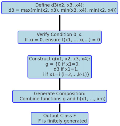
    Related Papers:

    [1] Yicang Zhou, Zhien Ma . Global stability of a class of discrete age-structured SIS models with immigration. Mathematical Biosciences and Engineering, 2009, 6(2): 409-425. doi: 10.3934/mbe.2009.6.409
    [2] Yan-Xia Dang, Zhi-Peng Qiu, Xue-Zhi Li, Maia Martcheva . Global dynamics of a vector-host epidemic model with age of infection. Mathematical Biosciences and Engineering, 2017, 14(5&6): 1159-1186. doi: 10.3934/mbe.2017060
    [3] Jianxin Yang, Zhipeng Qiu, Xue-Zhi Li . Global stability of an age-structured cholera model. Mathematical Biosciences and Engineering, 2014, 11(3): 641-665. doi: 10.3934/mbe.2014.11.641
    [4] Sara Y. Del Valle, J. M. Hyman, Nakul Chitnis . Mathematical models of contact patterns between age groups for predicting the spread of infectious diseases. Mathematical Biosciences and Engineering, 2013, 10(5&6): 1475-1497. doi: 10.3934/mbe.2013.10.1475
    [5] Georgi Kapitanov . A double age-structured model of the co-infection of tuberculosis and HIV. Mathematical Biosciences and Engineering, 2015, 12(1): 23-40. doi: 10.3934/mbe.2015.12.23
    [6] Zhisheng Shuai, P. van den Driessche . Impact of heterogeneity on the dynamics of an SEIR epidemic model. Mathematical Biosciences and Engineering, 2012, 9(2): 393-411. doi: 10.3934/mbe.2012.9.393
    [7] Guihong Fan, Yijun Lou, Horst R. Thieme, Jianhong Wu . Stability and persistence in ODE modelsfor populations with many stages. Mathematical Biosciences and Engineering, 2015, 12(4): 661-686. doi: 10.3934/mbe.2015.12.661
    [8] Yijun Lou, Bei Sun . Stage duration distributions and intraspecific competition: a review of continuous stage-structured models. Mathematical Biosciences and Engineering, 2022, 19(8): 7543-7569. doi: 10.3934/mbe.2022355
    [9] Shanjing Ren, Lingling Li . Global stability mathematical analysis for virus transmission model with latent age structure. Mathematical Biosciences and Engineering, 2022, 19(4): 3337-3349. doi: 10.3934/mbe.2022154
    [10] James M. Hyman, Jia Li . Epidemic models with differential susceptibility and staged progression and their dynamics. Mathematical Biosciences and Engineering, 2009, 6(2): 321-332. doi: 10.3934/mbe.2009.6.321
  • We study a class of functions F satisfying a condition denoted by 0x, meaning F(x)=0 whenever x meets a specific threshold. We show that F is generated by a finite set of functions, none of which are majority or choice functions. Key theoretical results are presented, including proofs of the closure of F under superposition and the inclusion FT0, where T0 denotes the set of all functions that evaluate to zero whenever at least one variable is zero. Our main theorems confirm that majority functions and choice functions are not elements of F. We further prove that F is finitely generated, that is, definable by a finite set of functions. These findings offer a novel framework for constructing finitely generated classes in multi-valued logic while excluding the commonly used but computationally intricate majority and choice functions, with practical implications in computational optimization. In conclusion, we discuss potential directions for further research, including the exploration of other classes of functions and the investigation of their properties and applications.


    Family planning involves consideration of the number (including the choice of zero) and spacing of children a family wishes to have. A number of factors can impact the family planning at the individual family level. At the population level the family planning and reproduction strategy including fertility, birth age and spacing of children, may be heavily influenced by economical conditions and societal resources which can be weighted heavily by the age-distribution of the entire population. In developing countries, policies like subsidizing education raise the earning power of women and the opportunity cost of having children, consequently lowers fertility [1]. Access to contraceptives may also yield lower fertility rates. In developed countries, the proportion of retired people is increasing, adding burden on the workforce population to support pensions and social programs. Increasing high skill migration may be an effective way to increase the return to education leading to lower fertility and a greater supply of highly skilled individuals [1], thus address the aging population problem.

    A well-known example of family planning and age-distribution of population being significantly regulated by political and social-economic consideration is the China's one-child policy implemented for many years. In 1973, the Chinese government issued voluntary guidelines on fertility control to encourage later marriage, longer spacing between births, and fewer births overall [2,3]. In 1981, China's National Family Planning Commission proposed a population control policy advocating one child per couple, which was moderated in 1984, allowing most rural families a second child [2,3,4]. In 2002, the policy was incorporated in the Population and Family Planning Law, at the same time, a second child was permitted in some provinces if both husband and wife were from single-child families [2,3,5]. In 2013, the policy was relaxed to allow a second child if either spouse was from a single-child family [3,6]. In October of 2015, the Chinese government announced a two-child policy, effective from January 1 of 2016 [7]. The new policy that allows each couple have two children was proposed in order to help address the population aging issue. It was reported that, starting from May 2018, Chinese authorities were in the process of ending the population control policies [8].

    A consequence of this recent change of the centralized population control policy after a long-term implementation of one-child per family policy is the obvious increasing of the family size, and substantial heterogeneity of the reproduction age and the spacing between the first and second child in those families with two children. This generates new close contact patterns in household and community level and thus any issue relevant to these contact patterns must be revisited. The control and prevention of childhood infectious diseases preventable by vaccine, such as pertussis, is one of these critical public health issues. Taking pertussis as an example, this childhood disease can be fatal in infants but infection can be prevented in other age groups with an effective vaccine. Pertussis vaccines wane over time, so those children who are expected to have younger siblings need to take a booster vaccine if (I) the prevalence of disease in the older age group and/or groups (recalling the potential heterogeneity of spacing between two children since females in multiple age groups may consider to give birth) is expected to be high; and (II) vaccine waning make this group of these groups less protected and more susceptible to the disease.

    To the best of my knowledge, there is no study on impact of family planning and the scale of density-regulated birth rate on the long-term population demographic distribution and childhood disease dynamics. However, there are a few studies which imply the impact of demographic change on infectious disease dynamics. These work include studies on demographic transition and the dynamics of measles in China [9], the influence of demographic change on spread of infectious diseases [10], the impact of demographic transition on rubella transmission dynamics in China [11], the effects of demographic change and immigration on infectious diseases in Italy [12], the effects of demographic change on disease transmission and vaccine impact in a household structured population [13], the dynamical consequences of demographic change in a model of disease transmission [14] and the impact of demographic change on the estimated future burden of hepatitis B and seasonal influenza in the Netherlands [15].

    This series of studies is dedicated to developing mathematical frameworks and analyses to examine the patterns of childhood infectious disease transmission, to identify prevalence of disease in different age groups, when female in multiple age intervals are giving birth to the second children. In this first paper of the series, we start with a simple stage-structured disease transmission model, and study the impact of family planning and the scale of density-regulated birth rate on the long-term population demographic distribution and infant disease incidence prevalence. We conduct our analyses by varying three parameters: birth rate, reproduction age interval(s), and the scale of the sub-population density regulation.

    In particular, we introduce a multi-stage (m-stages) stratified model, where the population is divided by age into m groups (stages) with the i-th age stage spanning the age interval of length τi. Assume that females in the age groups, k,k+1,,l-th groups give birth. For each group, we have the classical SIS epidemic-model, where the population is divided into the susceptible and the infectious. We consider the situation where the infectious period is much shorter than the period of each age stage. Therefore, the infectious individuals in the i-th age group Ii go back to the susceptible class Si before advancing to the (i+1)-th age group. The flowcharts of the demographic model and epidemiological model are shown in Figures 1 and 2 respectively.

    Figure 1.  Flow chart of the demographic model.
    Figure 2.  Flow chart of the epidemiological model.

    Let Si(t) be the population of the susceptible of the ith age group, Ii(t) be the population of the infectious of the ith age group. Ni(t) denotes the total population of the ith age group at time t. The death rate of the ith age group is given by μi; σ is the recover rate; the birth rate of the ith productive group is a nonlinear function bi(Ni); βij is the transmission rate of the disease from stage j to stage i. The age-stratified epidemiological model is given by the following equations:

    dS1(t)dt=li=kbi(Ni(t))li=kbi(Ni(tτ1))eμ1τ1μ1S1(t)mi=1β1iS1(t)Ii(t)+σI1(t)dSh(t)dt=li=kbi(Ni(th1j=1τj))eh1j=1μjτjli=kbi(Ni(thj=1τj))ehj=1μjτjμhSh(t)mi=1βhiSh(t)Ii(t)+σIh(t)for1<h<mdSm(t)dt=li=kbi(Ni(tm1j=1τj))em1j=1μjτjμmSm(t)mi=1βmiSm(t)Ii(t)+σIm(t)dIh(t)dt=mi=1βhiSh(t)Ii(t)σIh(t)μhIh(t)for1hm (1.1)

    The demographic model is given by

    dN1(t)dt=li=kbi(Ni(t))li=kbi(Ni(tτ1))eμ1τ1μ1N1(t)dNh(t)dt=li=kbi(Ni(th1j=1τj))eh1j=1μjτjli=kbi(Ni(thj=1τj))ehj=1μjτjμhNh(t)for1<h<mdNm(t)dt=li=kbi(Ni(tm1j=1τj))em1j=1μjτjμmNm(t). (1.2)

    In this section, we investigate the dynamics of the demographic model by studying the stability of equilibrium.

    Linearizing (1.2) at the zero equilibrium gives

    dN1(t)dt=li=kbi(0)Ni(t)li=kbi(0)Ni(tτ1)eμ1τ1μ1N1(t)dNh(t)dt=li=kbi(0)Ni(th1j=1τj)eh1j=1μjτjli=kbi(0)Ni(thj=1τj)ehj=1μjτjμhNh(t)for1<h<mdNm(t)dt=li=kbi(0)Ni(tm1j=1τj)em1j=1μjτjμmNm(t) (2.1)

    Let λ be eigenvalue of the linear system (2.1). By calculation, the characteristic equation is given by

    li=kbi(0)(1e(λ+μi)τi)eλi1j=1τji1j=1μjτjμi+λ=1 (2.2)

    Now we make the following assumption:

    (A1) The birth function takes the form bi(x)=pixq(x) where q(x) is a non-negative monotone decreasing function.

    Note that pi is the maximal number of children a female in age group i could give per unit time, q(x) is the function which implies the restriction of resources, so assumption (A1) reflects the ecological consideration that the reproduction is linear in x only for small densities and decreases as a consequence of intra specific competition. For example, one well known birth function which takes the form in assumption (A1) is the Ricker function b(x)=pxeqx.

    With this assumption, we have the following theorem on local stability of the zero equilibrium.

    Theorem 1. Under assumptions (A1), if li=kpiq(0)ei1j=1μjτj(1eμiτi)μi>1, then the zero equilibrium is unstable; if li=kpiq(0)ei1j=1μjτj(1eμiτi)μi<1, the zero equilibrium is stable.

    Proof. Let G(λ):=li=kbi(0)gi(λ), where gi(λ)=(1e(λ+μi)τi)eλi1j=1τji1j=1μjτjμi+λ. Then the characteristic equation (2.2) can be written as G(λ)=1. Calculating the derivative gives gi(λ)<0 on (μi,). Furthermore, gi(λ)0 as λ and gi(λ)+ as λμi. From assumption (A1), we have bi(0)=piq(0)>0. Therefore, G(λ) is monotone decreasing on (μ,) where μ=min{μi,i=k,k+1,...,l}. Moreover, G(λ)0 as λ and G(λ)+ as λμ.

    If G(0)=li=kpiq(0)ei1j=1μjτj(1eμiτi)μi>1, G(λ)>1, since G(λ) is monotone decreasing on (μ,) and limλG(λ)=0, the characteristic equation has a positive real root. So the zero equilibrium is unstable. If G(0)=li=kpiq(0)ei1j=1μjτj(1eμiτi)μi<1, G(λ)<1, since G(λ) is monotone decreasing on (μ,), limλG(λ)=0 and limλμG(λ)=+, the characteristic equation has a positive real root. So the zero equilibrium is stable.

    Suppose that there is a positive equilibrium (N1,N2,...,Nm), then we have

    li=kbi(Ni)li=kbi(Ni)eμ1τ1μ1N1=0li=kbi(Ni)eh1j=1μjτjli=kbi(Ni)ehj=1μjτjμhNh=0for1<h<mli=kbi(Ni)em1j=1μjτjμmNm=0 (2.3)

    From Eq (2.3) we derive

    N1=1μ1li=kbi(Ni)(1eμ1τ1)Nh=1μhli=kbi(Ni)eh1j=1μjτj(1eμhτh)for1<h<mNm=1μmli=kbi(Ni)em1j=1μjτj (2.4)

    The conditions for existence of this positive equilibrium is given in the following theorem.

    Theorem 2. Under assumption (A1) with limxq(x)=0, the positive equilibrium (N1,N2,...,Nm) exists and is unique if li=kpiq(0)ei1j=1μjτj(1eμiτi)μi>1.

    Proof. From Eq (2.4),

    Nh=μ1eh1j=1μjτj(1eμhτh)μh(1eμ1τ1)N1 (2.5)

    for khl. Equation (2.5) and the first equation in (2.4) imply that

    μ1N11eμ1τ1=li=kbi(μ1ei1j=1μjτj(1eμiτi)μi(1eμ1τ1)N1) (2.6)

    From assumption (A1), bi(x)=pixq(x), so Eq (2.6) becomes

    1=li=kpiei1j=1μjτj(1eμiτi)μiq(μ1ei1j=1μjτj(1eμiτi)μi(1eμ1τ1)N1) (2.7)

    So the positive equilibrium exists if there exists a positive N1 such that Eq (2.7) holds. Now let G(x)=li=kpiei1j=1μjτj(1eμiτi)μiq(μ1ei1j=1μjτj(1eμiτi)μi(1eμ1τ1)x). Since q(x) is monotone decreasing with respect to x, G(x) is monotone decreasing function. Furthermore, limxG(x)=0. So G(x)=1 has a unique positive solution if and only if G(0)>1, i.e., li=kpiq(0)ei1j=1μjτj(1eμiτi)μi>1.

    Note that Theorems 1 and 2 imply that the positive equilibrium exists and is unique if and only if the zero equilibrium is unstable.

    For the next, we study stability of this positive equilibrium.

    We denote by C+m the non-negative cone of the Banach space of continuous functions Cm={φ=(φ1,φ2,...,φm):[r,0]Rmcontinuous}, where r=max{τ1,τ2,...,τm}, i.e. C+m={φCm:φi(θ)0forθ[r,0],i=0,1,2,...,m}. By using the method of steps, it can be shown that for each φC+m, there is a unique solution of (1.2) π(φ,t)=(N1(φ,t),N2(φ,t),...,Nm(φ,t))R+m through φ that is well defined and satisfies π(φ;.)|[r,0]=φ.

    In fact, by taking integral and making substitutions, system (1.2) can be written as

    N1(t)=τ10eμ1θli=kbi(Ni(tθ))dθNh(t)=hj=1τjh1j=1τjli=kbi(Ni(tθ))eh1j=1μjτjμh(θh1j=1τj)dθ1<h<mNm(t)=m1j=1τjli=kbi(Ni(tθ))em1j=1μjτjμm(θm1j=1τj)dθ (2.8)

    In what follows, we give a preliminary result, then we give a theorem on global stability of the positive equilibrium.

    Lemma 1. Under assumption (A1), if the birth functions bi(x) are bounded for i=k,k+1,...,l, for every φC+m with φi(0)>0, i=1,2,...,m, the solution π(φ;t) of (1.2) is bounded above for t>0.

    Proof. Let N(t)=mi=1Ni(t). By adding up the m equations in Eq (1.2), we obtain

    dNdt=li=kbi(Ni(t))mi=1μiNi(t)li=kbi(Ni(t))μN(t)

    where μ is the smallest death rate in the m age groups, i.e., μ=min{μi,i=1,2,...,m}. Since the birth functions bi(x) are bounded for i=k,k+1,...,l, there are Mi for i=1,2,...,m such that bi(Ni(t))Mi. Let M=li=kMi, then dNdtMμN(t), which means that dNdt<0 when N>Mμ. So N is bounded, i.e., there is ˉN such that N(t)ˉN for t0. Therefore, Ni(t)ˉN for t0 for i=1,2,...,m. The solution π(φ;t) is bounded for t>0.

    Theorem 3. Under assumption (A1) with limxq(x)=0, if li=kpiq(0)ei1j=1μjτj(1eμiτi)μi>1 and li=k|bi(Ni)|ei1j=1μjτj(1+eμiτi)μi<1, then the positive equilibrium (N1,N2,...,Nm) is locally stable.

    Proof. The linearized equations at the endemic equilirbium (N1,N2,...,Nm) of system (1.2) is given by

    dN1(t)dt=li=kbi(Ni)Ni(t)li=kbi(Ni)Ni(tτ1)eμ1τ1μ1N1(t)dNh(t)dt=li=kbi(Ni)Ni(th1j=1τj)eh1j=1τjli=kbi(Ni)Ni(thj=1τj)ehj=1τjμhNh(t)for1<h<mdNm(t)dt=li=kbi(Ni)Ni(tm1j=1τj)em1j=1μjτjμmNm(t) (2.9)

    Let λ be eigenvalue of the linear system (2.9). By calculation, the characteristic equation is given by

    li=kbi(Ni)(1e(λ+μi)τi)eλi1j=1τji1j=1μjτjμi+λ=1 (2.10)

    Suppose that the characteristic equation (2.10) has an eigenvalue with non-negative real part, i.e., there exits λ=x+iy such that x0, then

    |bi(Ni)(1e(λ+μi)τi)eλi1j=1τji1j=1μjτjμi+λ|=|bi(Ni)(1e(x+iy+μi)τi)e(x+iy)i1j=1τji1j=1μjτjμi+x+iy||bi(Ni)||1e(x+iy+μi)τi||e(x+iy)i1j=1τji1j=1μjτj||μi+x+iy||bi(Ni)||1e(x+μi)τi(cosyτiisinyτi)||ei1j=1μjτj||μi+x+iy|=|bi(Ni)|(1e(x+μi)τicosyτi)2+(e(x+μi)τisinyτi)2|ei1j=1μjτj|(x+μi)2+y2|bi(Ni)|1+e2(x+μi)2e(x+μi)τicosyτi|ei1j=1μjτj|μi|bi(Ni)|1+e2(x+μi)+2e(x+μi)τi|ei1j=1μjτj|μi=|bi(Ni)|(1+e(x+μi)τi)ei1j=1μjτjμi|bi(Ni)|(1+eμiτi)ei1j=1μjτjμi (2.11)

    Therefore, Eq (2.10) and inequality (2.11) indicate that

    1=|li=kbi(Ni)(1e(λ+μi)τi)eλi1j=1τji1j=1μjτjμi+λ|li=k|bi(Ni)(1e(λ+μi)τi)eλi1j=1τji1j=1μjτjμi+λ|li=k|bi(Ni)|(1+eμiτi)ei1j=1μjτjμi (2.12)

    which contradicts with the assumption that li=k|bi(Ni)|ei1j=1μjτj(1+eμiτi)μi<1. So the characteristic equation (2.10) has no eigenvalue with non-negative real part, the positive equilibrium (N1,N2,...,Nm) is locally stable.

    Theorem 4. Under assumption (A1) with limxq(x)=0 and the birth functions bi(x) bounded for i=k,k+1,...,l, assume that μh=μ and τh=τ for some μ>0, τ>0 and all khl. If li=k|bi(Ni)|ei1j=1μjτj(1+eμiτi)μi<1, then the positive equilibrium (N1,N2,...,Nm) is globally stable. i.e., limtπ(φ;t)=(N1,N2,...,Nm) for φC+m with φi(0)>0.

    Proof. Let {Ni(t)} be a solution of Eq (1.2). Since it's bounded, we can define

    δi=lim inftNi(t),γi=lim suptNi(t)

    Let h be such that khl, i.e. Nh is a productive group. There exists a sequence {tn} and a sequence {sn} such that limnNh(tn)=γh and limnNh(sn)=δh. So there exists some ϵ>0 such that δiϵ<Ni(tn)<γi+ϵ and δiϵ<Ni(sn)<γi+ϵ for n large enough for all kil.

    From the integrated equation (2.8),

    Nh(tn)<hj=1τjh1j=1τjli=kpi(γi+)q(δi)eh1j=1μjτjμh(θh1j=1τj)dθ

    Let n and ϵ0, the inequality becomes

    γhhj=1τjh1j=1τjli=kpiγiq(δi)eh1j=1μjτjμh(θh1j=1τj)dθ=li=kpiγiq(δi)eh1j=1μjτj+μhh1j=1τjhj=1τjh1j=1τjeμhθdθ=li=kpiγiq(δi)(1eμhτh)eh1j=1μjτjμhq(δi) (2.13)

    Now let A:=li=kpiγiq(δi), Eq (2.13) implies that

    A=li=kpiγiq(δi)li=kpiA(1eμiτi)ei1j=1μjτjμiq(δi)

    which further implies that

    li=kpiq(δi)(1eμiτi)ei1j=1μjτjμi1 (2.14)

    Let B:=li=kpiNiq(Ni), from Eq (2.4)

    B = \sum\limits_{i = k}^{l}p_{i}N_{i}^{*}q(N_{i}^{*}) = \sum\limits_{i = k}^{l}p_{i}B\frac{(1-e^{-\mu_{i}\tau_{i}})e^{-\sum_{j = 1\;}^{i-1}\mu_{j}\tau_{j}}}{\mu_{i}}q(N_{i}^{*})

    so

    \sum\limits_{i = k}^l {{p_i}} \frac{{(1 - {e^{ - {\mu _i}{\tau _i}}}\;){e^{ - \sum_{j = 1\;}^{i - 1} {\;\;{\mu _j}} {\tau _j}}}}}{{{\mu _i}}}q(N_i^*) = 1 (2.15)

    From assumption (A1), q(x) is monotone decreasing, then Eqs (2.14) and (2.15) imply that there exists h_{1} such that k\leq h_{1}\leq l and \delta_{h_{1}}\leq N_{h_{1}}^{*} . From the integrated equation (2.8),

    N_{h}(s_{n}) \gt \int_{\sum_{j = 1\;}^{h-1}\tau_{j}}^{\sum_{j = 1\;}^{h}\tau_{j}}\sum\limits_{i = k}^{l}p_{i}(\delta_{i}-\epsilon)q(\gamma_{i}+\epsilon)e^{-\sum_{j = 1\;}^{h-1}\mu_{j}\tau_{j}-\mu_{h}(\theta-\sum_{j = 1\;}^{h-1}\tau_{j})}\;d\theta

    Following similar calculation as inequalities (2.13) and (2.14), we obtain

    \begin{equation} \sum\limits_{i = k}^{l}p_{i}q(\gamma_{i})\frac{(1-e^{-\mu_{i}\tau_{i}})e^{-\sum_{j = 1\;}^{i-1}\mu_{j}\tau_{j}}}{\mu_{i}}\leq1. \end{equation} (2.16)

    From assumption (A1), q(x) is monotone decreasing, then Eqs (2.15) and (2.16) imply that there exists h_{2} such that k\leq h_{2}\leq l and \gamma_{h_{2}}\geq N_{h_{2}}^{*} .

    By substituting variables, from Eqs (2.4) and (2.8) we obtain

    \begin{equation} (N_{k}(t)-N_{k}^{*})e^{\sum_{j = 1\;}^{k-1}\mu_{j}\tau_{j}} = \int_{\sum_{j = 1\;}^{k-1}\tau_{j}}^{\sum_{j = 1\;}^{k}\tau_{j}}\sum\limits_{i = k}^{l}(b_{i}(N_{i}(t-\theta)-b_{i}(N_{i}^{*}))e^{-\mu_{k}(\theta-\sum_{j = 1\;}^{k-1}\tau_{j})}d\theta \end{equation} (2.17)

    and

    \begin{equation} (N_{h}(t)-N_{h}^{*})e^{\sum_{j = 1\;}^{h-1}\mu_{j}\tau_{j}} = \int_{\sum_{j = 1\;}^{k-1}\tau_{j}}^{\sum_{j = 1\;}^{k-1}\tau_{j}+\tau_{h}}\sum\limits_{i = k}^{l}(b_{i}(N_{i}(t-\theta)-b_{i}(N_{i}^{*}))e^{-\mu_{h}(\theta-\sum_{j = 1\;}^{k-1}\tau_{j})}d\theta \end{equation} (2.18)

    Since \mu_{h} = \mu and \tau_{h} = \tau for k\leq h\leq l , Eqs (2.17) and (2.18) imply that

    \begin{equation} (N_{k}(t)-N_{k}^{*})e^{\sum_{j = 1\;}^{k-1}\mu_{j}\tau_{j}} = (N_{h}(t)-N_{h}^{*})e^{\sum_{j = 1\;}^{h-1}\mu_{j}\tau_{j}} \end{equation} (2.19)

    for k\leq h\leq l .

    Scenario 1: \gamma_{k} = N_{k}^{*}

    In this scenario, since the positive equilibrium is locally stable, \delta_{k} = \gamma_{k} = N_{k}^{*} , and \lim_{t\rightarrow\infty}N_{k}(t) = N_{k}^{*} . From Eq (2.19), \lim_{t\rightarrow\infty}N_{h}(t) = N_{h}^{*} for all k\leq h\leq l .

    Scenario 2: \gamma_{k} > N_{k}^{*}

    In this scenario, since the positive equilibrium is locally stable, \delta_{k} > N_{k}^{*} , then N_{k}(t) > N_{k}^{*} for t large enough. From Eq (2.19), N_{h_{1}}(t) > N_{h_{1}}^{*} for t large enough, which means that \delta_{h_{1}}\geq N_{h_{1}}^{*} . Since we have \delta_{h_{1}}\leq N_{h_{1}}^{*} from previous discussion, \delta_{h_{1}} = N_{h_{1}}^{*} . Therefore, \delta_{h_{1}} = \gamma_{h_{1}} = N_{h_{1}}^{*} , i.e., \lim_{t\rightarrow\infty}N_{h_{1}}(t) = N_{h_{1}}^{*} . From Eq (2.19), \lim_{t\rightarrow\infty}N_{h}(t) = N_{h}^{*} for all k\leq h\leq l .

    Scenario 3: \gamma_{k} < N_{k}^{*}

    Then \delta_{k} < N_{k}^{*} and N_{k}(t) < N_{k}^{*} for t large enough. From Eq (2.19), N_{h_{2}}(t) < N_{h_{2}}^{*} for t large enough, which implies that \gamma_{h_{2}}\leq N_{h_{2}}^{*} . Since we have \gamma_{h_{2}}\geq N_{h_{2}}^{*} from previous discussion, \gamma_{h_{2}} = N_{h_{2}}^{*} . i.e., \lim_{t\rightarrow\infty}N_{h_{2}}(t) = N_{h_{2}}^{*} . From Eq (2.19), \lim_{t\rightarrow\infty}N_{h}(t) = N_{h}^{*} for all k\leq h\leq l .

    From discussion above, \lim_{t\rightarrow\infty}N_{h}(t) = N_{h}^{*} for all k\leq h\leq l . Then by the integral equation (2.8), \lim_{t\rightarrow\infty}N_{h}(t) = N_{h}^{*} for all 1\leq h\leq m .

    Now we focus on the epidemic model, which is an ODE system given by

    \begin{equation} \frac{dI_{h}(t)}{dt} = \sum\limits_{i = 1}^{m}\beta_{hi}(N_{h}(t)-I_{h}(t))I_{i}(t)-\sigma I_{h}(t)-\mu_{h}I_{h}(t)\; {}\mbox{for}\; {}1\leq h\leq m \end{equation} (3.1)

    Note that Eq (3.1) is derived from the last equation in (1.1) by replacing S_{h}(t) by N_{h}(t)-I_{h}(t) .

    Suppose that the population has reached the positive equilibrium, then system (3.1) is given by

    \begin{equation} \frac{dI_{h}(t)}{dt} = \sum\limits_{i = 1}^{m}\beta_{hi}(N_{h}^{*}-I_{h}(t))I_{i}(t)-\sigma I_{h}(t)-\mu_{h}I_{h}(t)\; {}\mbox{for}\; {}1\leq h\leq m \end{equation} (3.2)

    Let \mathbf{I} = (I_{1}, I_{2}, ..., I_{m})^{T} , the flow of the solution of system (3.2) with initial value \mathbf{I^{0}} = (I_{1}^{0}, I_{2}^{0}, ..., I_{m}^{0}) is given by \phi_{t}(\mathbf{I^{0}}) . Let V = (0, N_{1}^{*})\times(0, N_{2}^{*})\times...\times(0, N_{m}^{*}) . We have the following conclusion

    Theorem 5. If \mathbf{I}_{i}^{0}\in(0, N_{i}^{*}) , then \phi_{ti}(\mathbf{I^{0}})\in(0, N_{i}^{*}) , i.e., V is invariant under the flow \phi_{t} .

    Proof. Suppose that there is a smallest t_{0} such that there is j\in\{1, 2, ..., m\} such that I_{j}(t_{0}) = 0 . Since \mathbf{I}(t) is not constant 0, we have \frac{dI_{j}(t)}{dt}|_{t = t_{0}} = \sum_{i = 1}^{m}\beta_{hi}(N_{h}^{*}-I_{h}(t_{0}))I_{i}(t_{0}) > 0 . On the other hand, since t_{0} is the smallest s.t. I_{j}(t_{0}) = 0 , \frac{dI_{j}(t)}{dt}|_{t = t_{0}} = \lim_{\epsilon\rightarrow0}\frac{I_{j}(t_{0}-\epsilon)-I_{j}(t_{0})}{-\epsilon}\leq0 , which is a contradiction. So I_{j}(t) > 0 for all 1\leq j\leq m and all t > 0 with initial value in V .

    Similarly, suppose that there is a smallest t_{0} such that there is j\in\{1, 2, ..., m\} such that I_{j}(t_{0}) = N_{j}^{*} , then from Eq (3.2), \frac{dI_{j}}{dt}|_{t = t_{0}} = -\sigma I_{h}(t_{0})-\mu_{h}I_{h}(t_{0}) < 0 . On the other hand, since t_{0} is the smallest s.t. I_{j}(t_{0}) = N_{j}^{*} , \frac{dI_{j}(t)}{dt}|_{t = t_{0}} = \lim_{\epsilon\rightarrow0}\frac{I_{j}(t_{0}-\epsilon)-I_{j}(t_{0})}{-\epsilon}\geq0 , which is a contradiction. So I_{j}(t) < 0 for all 1\leq j\leq m and all t > 0 with initial value in V .

    Equation (3.2) has (0, 0, ..., 0) as the disease-free equilibrium. Linearization around this equilibrium gives the following linear system

    \begin{equation} \frac{dI_{h}(t)}{dt} = \sum\limits_{i = 1}^{m}\beta_{hi}N_{h}^{*}I_{i}(t)-\sigma I_{h}(t)-\mu_{h}I_{h}(t) \end{equation} (3.3)

    for 1\leq h\leq m Following the method in [16], we get

    F = \begin{bmatrix} \beta_{11}N_{1}^{*}&\beta_{12}N_{1}^{*}&\cdots &\beta_{1m}N_{1}^{*} \\ \beta_{21}N_{2}^{*}&\beta_{22}N_{2}^{*}&\cdots &\beta_{2m}N_{2}^{*} \\ \vdots & \vdots & \ddots & \vdots\\ \beta_{m1}N_{m}^{*}&\beta_{m2}N_{m}^{*}&\cdots &\beta_{mm}N_{m}^{*} \end{bmatrix}

    and

    V = \begin{bmatrix} \sigma+\mu_{1}&0&\cdots &0 \\ 0&\sigma+\mu_{2}&\cdots &0 \\ \vdots & \vdots & \ddots & \vdots\\ 0&0&\cdots &\sigma+\mu_{m} \end{bmatrix}

    Then we have

    FV^{-1} = \begin{bmatrix} \frac{\beta_{11}N_{1}^{*}}{\sigma+\mu_{1}}&\frac{\beta_{12}N_{1}^{*}}{\sigma+\mu_{2}}&\cdots &\frac{\beta_{1m}N_{1}^{*}}{\sigma+\mu_{m}} \\ \frac{\beta_{21}N_{2}^{*}}{\sigma+\mu_{1}}&\frac{\beta_{22}N_{2}^{*}}{\sigma+\mu_{2}}&\cdots &\frac{\beta_{2m}N_{2}^{*}}{\sigma+\mu_{m}} \\ \vdots & \vdots & \ddots & \vdots\\ \frac{\beta_{m1}N_{m}^{*}}{\sigma+\mu_{1}}&\frac{\beta_{m2}N_{m}^{*}}{\sigma+\mu_{2}}&\cdots &\frac{\beta_{mm}N_{m}^{*}}{\sigma+\mu_{m}} \end{bmatrix}

    In particular, if we assume that \beta_{ij} = \alpha_{i}\lambda_{j} , it can be calculated from induction that the characteristic equation of FV^{-1} is given by \lambda^{m-1}(\lambda-\sum_{i = 1}^{m}\frac{\alpha_{i}\lambda_{i}N_{i}^{*}}{\sigma+\mu_{i}}) = 0 , then

    R_{0} = \rho(FV^{-1}) = \sum\limits_{i = 1}^{m}\frac{\alpha_{i}\lambda_{i}N_{i}^{*}}{\sigma+\mu_{i}}

    The following theorem follows

    Theorem 6. Assume that \beta_{ij} = \alpha_{i}\lambda_{j} . Then when \sum_{i = 1}^{m}\frac{\alpha_{i}\lambda_{i}N_{i}^{*}}{\sigma+\mu_{i}} < 1 , the disease-free equilibrium of system (3.2) is stable; when \sum_{i = 1}^{m}\frac{\alpha_{i}\lambda_{i}N_{i}^{*}}{\sigma+\mu_{i}} > 1 , the disease-free equilibrium of system (3.2) is unstable.

    For the assumption \beta_{ij} = \alpha_{i}\lambda_{j} , if we assume that the population is homogeneously mixed, \alpha_{i} can be interpreted as susceptibility of age group i and \lambda_{j} can be interpreted as infectivity of age group j .

    Suppose system (3.2) has a nontrivial equilibrium (I_{1}^{*}, I_{2}^{*}, ..., I_{m}^{*}) , by plugging in the Eq (3.2) we derive

    \begin{equation} \sum\limits_{i = 1}^{m}\beta_{hi}(N_{h}^{*}-I_{h}^{*})I_{i}^{*}-\sigma I_{h}^{*}-\mu_{h}I_{h}^{*} = 0 \end{equation} (3.4)

    for 1\leq h\leq m . In particular, if we assume that \beta_{ij} = \alpha_{i}\lambda_{j} , then Eq (3.4) can be written as

    \begin{equation} (N_{h}^{*}-I_{h}^{*})\sum\limits_{i = 1}^{m}\alpha_{h}\lambda_{i}I_{i}^{*}-\sigma I_{h}^{*}-\mu_{h}I_{h}^{*} = 0 \end{equation} (3.5)

    for 1\leq h\leq m . From Eq (3.5) we get

    \begin{equation} \sum\limits_{i = 1}^{m}\lambda_{i}I_{i}^{*} = \frac{(\sigma+\mu_{h})I_{h}^{*}}{\alpha_{h}(N_{h}^{*}-I_{h}^{*})} \end{equation} (3.6)

    for 1\leq h\leq m . and

    \frac{\sigma+\mu_{h}}{\alpha_{h}(N_{h}^{*}/I_{h}^{*}-1)} = \frac{\sigma+\mu_{1}}{\alpha_{1}(N_{1}^{*}/I_{1}^{*}-1)}

    Now let M_{i} = \frac{N_{i}^{*}}{I_{i}^{*}}-1 and l_{i} = \frac{\sigma+\mu_{i}}{\alpha_{i}} , then

    \frac{l_{i}}{M_{i}} = \frac{l_{1}}{M_{1}}

    Plugging I_{i}^{*} = \frac{N_{i}^{*}}{M_{i}+1} into Eq (3.6) with h = 1 , we have

    \sum\limits_{i = 1}^{m}\frac{\lambda_{i}N_{i}^{*}}{M_{i}+1} = \frac{l_{1}}{M_{1}}

    It follows that

    \sum\limits_{i = 1}^{m}\frac{\lambda_{i}N_{i}^{*}}{l_{i}+l_{1}/M_{1}} = 1

    Now define G:(0, N_{1}^{*})\longrightarrow\mathbb{R} by

    \begin{equation} G(x) = \sum\limits_{i = 1}^{m}\frac{\lambda_{i}N_{i}^{*}}{l_{i}+l_{1}/M} \end{equation} (3.7)

    where M = \frac{N_{1}^{*}}{x}-1 . Then I_{1}^{*} is a solution of G(x) = 1 .

    Note that G(x) is monotone non-increasing with respect to x , G(x)\longrightarrow 0 as x\longrightarrow N_{1}^{*} and G(x)\longrightarrow \sum_{i = 1}^{m}\frac{\lambda_{i}N_{i}^{*}}{l_{i}} as x\longrightarrow 0 . So G(x) = 1 has a solution in (0, N_{1}^{*}) if and only if \sum_{i = 1}^{m}\frac{\lambda_{i}N_{i}^{*}}{l_{i}} > 1 , and the solution is unique by monotonicity of G(x) .

    Note that R_{0} = \sum_{i = 1}^{m}\frac{\lambda_{i}N_{i}^{*}}{l_{i}} . We conclude that

    Theorem 7. Assume that \beta_{ij} = \alpha_{i}\lambda_{j} . The endemic equilibrium of system (3.2) exists and is unique if and only if R_{0} = \sum_{i = 1}^{m}\frac{\lambda_{i}N_{i}^{*}}{l_{i}} > 1 .

    Now we state the following theorem on global stability of the endemic equilibrium.

    Theorem 8. Assume that \beta_{ij} = \alpha_{i}\lambda_{j} .Let V = (0, N_{1}^{*})\times(0, N_{2}^{*})\times...\times(0, N_{m}^{*}) . If R_{0} > 1 , then the endemic equilibrium \{I_{i}^{*}\} of system (3.2) attracts all the forward orbits going through V .

    Proof. Let F:V\longrightarrow\mathbb{R}^{m} be defined by F_{h}(I_{1}, I_{2}, ..., I_{m}) = \sum_{i = 1}^{m}\beta_{hi}(N_{h}^{*}-I_{h})I_{i}-\sigma I_{h}-\mu_{h}I_{h} .

    It suffices to prove that

    (H1) System (3.2) is cooperative, i.e., \frac{\partial F_{h}}{\partial I_{j}}\geq0 for h\neq j .

    (H2) F is irreducible in the sense that the matrix [\frac{\partial F_{h}}{\partial I_{j}}] is irreducible.

    (H3) Solutions of Eq (3.2) with initial value (I_{1}^{0}, I_{2}^{0}, ..., I_{m}^{0}) such that \left\vert I_{h}^{0}\right\vert\leq N_{h}^{*} are bounded.

    Then by Theorems 1.5 and 2.4 in [17], (H1) and (H2) imply that system (3.2) doesn't have a non-constant periodic solution. By Theorem 1.1 in [17], (H1) and (H2) also imply that the solution flows of Eq (3.2) going through V have positive derivatives. Then by Theorem 4.1 in [17] and (H3) we conclude that almost all forward orbits of V converge to the endemic equilibrium \{I_{i}^{*}\} .

    (H1) \frac{\partial F_{h}}{\partial I_{j}} = \beta_{hj}(N_{h}^{*}-I_{h}) > 0 for h\neq j .

    (H2) \frac{\partial F_{h}}{\partial I_{h}} = \beta_{hh}(N_{h}^{*}-I_{h})-\sum_{i = 1}^{m}\beta_{hi}I_{i}-\sigma-\mu_{h} . Now let A = [\frac{\partial F_{h}}{\partial I_{j}}] . A_{hj} = \frac{\partial F_{h}}{\partial I_{j}} > 0 for h\neq j by (H1). Suppose there is 1\leq h\leq m such that A_{hh}\leq0 , A_{hh}^{2} = \sum_{i = 1}^{m}A_{hi}A_{ih} > 0 . Therefore, for each pair of indices h and j , there exists a natural number n such that A_{hj}^{n} is positive, which implies that the matrix A is irreducible.

    (H3) It can be derived directly from Theorem 5.

    Now if we look back on the original epidemic model (3.1), we have the following Theorem from Theorem 8.

    Theorem 9. Under assumption (A1) with \lim_{x\rightarrow\infty}q(x) = 0 , assume that \beta_{ij} = \alpha_{i}\lambda_{j} and \mu_{h} = \mu , \tau_{h} = \tau for some \mu > 0 , \tau > 0 and all k\leq h\leq l .Let V = (0, N_{1}^{*})\times(0, N_{2}^{*})\times...\times(0, N_{m}^{*}) . If \sum_{i = k}^{l}\frac{\left\vert b_{i}'(N_{i}^{*})\right\vert e^{-\sum_{j = 1\;}^{i-1}\mu_{j}\tau_{j}}(1+e^{-\mu_{i}\tau_{i}})}{\mu_{i}} < 1 and R_{0} > 1 , then \{I_{i}^{*}\} attracts all the forward orbits going through V in system (3.1).

    Proof. From Theorem 4, \lim_{t\rightarrow\infty}N_{h}(t) = N_{h}^{*} for all 1\leq h\leq m . Denote \Phi(t, s, x_{0}) the solution of system (3.1) with x(s) = x_{0} , and denote \Theta(t, x_{0}) the solution of system (3.2) with y(0) = x_{0} . Then by Proposition 1.1 in [18], \Phi is asymptotically autonomous semiflow with limit semiflow \Theta . Let \mathcal{O}_{\Phi}(s, x) = \{\Phi(t, s, x): t\geq s\} , x\in V , then \mathcal{O}_{\Phi}(s, x) has compact closure in V since it's bounded. Let \omega = \omega(s, x) which is the \omega -limit set of \mathcal{O}_{\Phi}(s, x) . By Theorem 1.8 in [18], we conclude that \omega is non-empty, compact and connected, and it attracts \Phi(t, s, x) . Moreover, \omega is invariant for the semiflow \Theta and is chain recurrent for \Theta .

    Now suppose that \omega\neq\{I_{i}^{*}\} . There exists x = (x_{1}, x_{2}, ..., x_{m})\in \omega such that x\neq\{I_{i}^{*}\} . Let \epsilon = d(x, \{I_{i}^{*}\}) . Since \omega is compact, there exists T > 0 such that d(\Theta(t, x_{0}), \{I_{i}^{*}\}) < \frac{\epsilon}{2} for all x_{0}\in\omega and t\geq T . By the definition of chain recurrence, there is an (\frac{\epsilon}{2}, T) chain from x to x , i.e., there is a sequence \{x = x_{1}, x_{2}, ..., x_{n+1} = x; t_{1}, t_{2}, ..., t_{n}\} for x_{i}\in\omega and t_{i}\geq T such that d(\Theta(t_{i}, x_{i}), x_{i+1}) < \frac{\epsilon}{2} . Then d(\Theta(t_{n}, x_{n}), x) < \frac{\epsilon}{2} , which indicates that d(x, \{I_{i}^{*}\})\leq d(\Theta(t_{n}, x_{n}), x)+d(\Theta(t_{n}, x_{n}), \{I_{i}^{*}\}) < \frac{\epsilon}{2}+\frac{\epsilon}{2} = \epsilon , which contradicts with \epsilon = d(x, \{I_{i}^{*}\}) . Therefore, \omega = \{I_{i}^{*}\} , i.e., \{I_{i}^{*}\} attracts all the forward orbits going through V in system (3.1).

    In this section, we assume that the birth rate of age group i is given by b_{i}(N_{i}) = p_{i}N_{i}e^{-qN} , we'll analyze how do demographic distribution \frac{N_{i}^{*}}{N} and infant disease rate at endemic equilibrium \frac{I_{1}^{*}}{N_{1}^{*}} change with birth parameters p_{i} , q and productive age k .

    By plugging b_{i}(N_{i}) = p_{i}N_{i}e^{-qN} into Eq (2.4), we have

    \sum\limits_{i = k}^{l}p_{i}N_{i}^{*}e^{-qN} = \frac{\mu_{h}N_{h}^{*}}{e^{-\sum_{j = 1\;}^{h-1}\mu_{j}\tau_{j}}(1-e^{-\mu_{h}\tau_{h}})}

    for 1\leq h\leq m .

    \frac{N_{i}^{*}}{N_{h}^{*}} = \frac{\mu_{h}e^{-\sum_{j = 1\;}^{i-1}\mu_{j}\tau_{j}}(1-e^{-\mu_{i}\tau_{i}}\;)}{\mu_{i}e^{-\sum_{j = 1\;}^{h-1}\mu_{j}\tau_{j}}(1-e^{-\mu_{h}\tau_{h}}\;)}

    for 1 < i, h < m . Combine the above two formulas, we have

    \sum\limits_{i = k}^{l}p_{i}\frac{\mu_{h}e^{-\sum_{j = 1\;}^{i-1}\mu_{j}\tau_{j}}(1-e^{-\mu_{i}\tau_{i}}\;)}{\mu_{i}e^{-\sum_{j = 1\;}^{h-1}\mu_{j}\tau_{j}}(1-e^{-\mu_{h}\tau_{h}})}N_{h}^{*}e^{-qN} = \frac{\mu_{h}N_{h}^{*}}{e^{-\sum_{j = 1\;}^{h-1}\mu_{j}\tau_{j}}(1-e^{-\mu_{h}\tau_{h}}\;)}

    Thus

    \sum\limits_{i = k}^{l}\frac{p_{i}e^{-\sum_{j = 1\;}^{i-1}\mu_{j}\tau_{j}}(1-e^{-\mu_{i}\tau_{i}})}{\mu_{i}} = e^{qN}

    Solving for N gives

    \begin{equation} N = \frac{1}{q}In\sum\limits_{i = k}^{l}\frac{p_{i}e^{-\sum_{j = 1\;}^{i-1}\mu_{j}\tau_{j}}(1-e^{-\mu_{i}\tau_{i}})}{\mu_{i}} \end{equation} (4.1)

    From Eq (2.4), we define

    Q: = \frac{\mu_{1}N_{1}^{*}}{1-e^{-\mu_{1}\tau_{1}}} = \frac{\mu_{h}N_{h}^{*}}{e^{-\sum_{j = 1\;}^{h-1}\mu_{j}\tau_{j}}(1-e^{-\mu_{h}\tau_{h}})} = \frac{\mu_{m}N_{m}^{*}}{e^{-\sum_{j = 1\;}^{m-1}\mu_{j}\tau_{j}}}

    for 1\leq h\leq m . It follows that

    \begin{equation} \begin{aligned} N_{1}^{*}& = \frac{1-e^{-\mu_{1}\tau_{1}}}{\mu_{1}}Q\\ N_{h}^{*}& = \frac{e^{-\sum_{j = 1\;}^{h-1}\mu_{j}\tau_{j}}(1-e^{-\mu_{h}\tau_{h}})}{\mu_{h}}Q\; {}\; {}\mbox{for}\; {}1 \lt h \lt m\\ N_{m}^{*}& = \frac{e^{-\sum_{j = 1\;}^{m-1}\mu_{j}\tau_{j}}}{\mu_{m}}Q \end{aligned} \end{equation} (4.2)

    By plugging Eq (4.2) into N = \sum_{h = 1}^{m}N_{h}^{*} , we have

    \begin{equation} N = (\frac{1-e^{-\mu_{1}\tau_{1}}}{\mu_{1}}+\sum\limits_{h = 1}^{m-1}\frac{e^{-\sum_{j = 1\;}^{h-1}\mu_{j}\tau_{j}}(1-e^{-\mu_{h}\tau_{h}})}{\mu_{h}}+\frac{e^{-\sum_{j = 1\;}^{m-1}\mu_{j}\tau_{j}}}{\mu_{m}})Q \end{equation} (4.3)

    Equations (4.2) and (4.3) give

    \begin{equation} \begin{aligned} \frac{N_{1}^{*}}{N}& = \frac{\frac{1-e^{-\mu_{1}\tau_{1}}}{\mu_{1}}}{\frac{1-e^{-\mu_{1}\tau_{1}}}{\mu_{1}}+\sum_{h = 1}^{m-1}\frac{e^{-\sum_{j = 1\;}^{h-1}\mu_{j}\tau_{j}}(1-e^{-\mu_{h}\tau_{h}})}{\mu_{h}}+\frac{e^{-\sum_{j = 1\;}^{m-1}\mu_{j}\tau_{j}}}{\mu_{m}}}\\ \frac{N_{h}^{*}}{N}& = \frac{\frac{e^{-\sum_{j = 1\;}^{h-1}\mu_{j}\tau_{j}}(1-e^{-\mu_{h}\tau_{h}})}{\mu_{h}}}{\frac{1-e^{-\mu_{1}\tau_{1}}}{\mu_{1}}+\sum_{h = 1}^{m-1}\frac{e^{-\sum_{j = 1\;}^{h-1}\mu_{j}\tau_{j}}(1-e^{-\mu_{h}\tau_{h}})}{\mu_{h}}+\frac{e^{-\sum_{j = 1\;}^{m-1}\mu_{j}\tau_{j}}}{\mu_{m}}}\; {}\; {}\mbox{for}\; {}1 \lt h \lt m\\ \frac{N_{m}^{*}}{N}& = \frac{\frac{e^{-\sum_{j = 1\;}^{m-1}\mu_{j}\tau_{j}}}{\mu_{m}}}{\frac{1-e^{-\mu_{1}\tau_{1}}}{\mu_{1}}+\sum_{h = 1}^{m-1}\frac{e^{-\sum_{j = 1\;}^{h-1}\mu_{j}\tau_{j}}(1-e^{-\mu_{h}\tau_{h}})}{\mu_{h}}+\frac{e^{-\sum_{j = 1\;}^{m-1}\mu_{j}\tau_{j}}}{\mu_{m}}} \end{aligned} \end{equation} (4.4)

    It's obvious from Eq (4.4) that change of p_{i} , q and k don't make a change on the demographic distribution \frac{N_{h}^{*}}{N} for 1\leq h\leq m .

    Proposition 10. Assume that the birth rate of age group i is given by b_{i}(N_{i}) = p_{i}N_{i}e^{-qN} . The stablized demographic distribution N_{h}^{*}/N doesn't change with birth parameters p_{i} , q and reproductive age k .

    Note that change of p_{i} , q and k does have an impact on the total number N and N_{h}^{*} , though they don't influence the ratio N_{h}^{*}/N .

    It can be seen from Eq (4.1) that N increases as p_{i} increases, decreases as q or k increases, so does N_{h}^{*} for all 1\leq h\leq m .

    Now we study the impact of changes of p_{i} , q and k on the infant disease rate \frac{I_{1}^{*}}{N_{1}^{*}} .

    In the last section, we get that when R_{0} > 1 , there is a endemic equilibrium of system 3.2 where I_{1}^{*} satisfies \sum_{i = 1}^{m}\frac{\lambda_{i}\frac{N_{i}^{*}}{N}N}{l_{i}+\frac{l_{1}}{M_{1}}} = 1 where l_{i} = \frac{\sigma+\mu_{i}}{\alpha_{i}} and M_{i} = \frac{N_{i}^{*}}{I_{i}^{*}}-1 . By taking derivative with respect to q , we get

    \sum\limits_{i = 1}^{m}\frac{\lambda_{i}\frac{N_{i}^{*}}{N}\frac{dN}{dq}(l_{i}+\frac{l_{1}}{M_{1}})+\frac{l_{1}}{M_{1}^{2}}\frac{dM_{1}}{dq}\lambda_{i}N_{i}^{*}}{(l_{i}+\frac{l_{1}}{M_{1}})^{2}} = 0

    So

    \begin{equation} \frac{dM_{1}}{dq} = -\sum\limits_{i = 1}^{m}\frac{\lambda_{i}\frac{N_{i}^{*}}{N}\frac{dN}{dq}(l_{i}+\frac{l_{1}}{M_{1}})}{(l_{i}+\frac{l_{1}}{M_{1}})^{2}}/\sum\limits_{i = 1}^{m}\frac{\frac{l_{1}}{M_{1}^{2}}\lambda_{i}N_{i}^{*}}{(l_{i}+\frac{l_{1}}{M_{1}})^{2}} \gt 0 \end{equation} (4.5)

    which means that \frac{N_{1}^{*}}{I_{1}^{*}} increases as q increases, so \frac{I_{1}^{*}}{N_{1}^{*}} decreases as q increases.

    Similarly, we have

    \begin{equation} \frac{dM_{1}}{dp_{i}} = -\sum\limits_{i = 1}^{m}\frac{\lambda_{i}\frac{N_{i}^{*}}{N}\frac{dN}{dp_{i}}(l_{i}+\frac{l_{1}}{M_{1}})}{(l_{i}+\frac{l_{1}}{M_{1}})^{2}}/\sum\limits_{i = 1}^{m}\frac{\frac{l_{1}}{M_{1}^{2}}\lambda_{i}N_{i}^{*}}{(l_{i}+\frac{l_{1}}{M_{1}})^{2}} \lt 0 \end{equation} (4.6)

    which means that \frac{N_{1}^{*}}{I_{1}^{*}} decreases as p_{i} increases, so \frac{I_{1}^{*}}{N_{1}^{*}} increases as p_{i} increases.

    If k gets larger, N gets smaller as discussed above, \frac{N_{i}^{*}}{N} doesn't change, since we have \sum_{i = 1}^{m}\frac{\lambda_{i}\frac{N_{i}^{*}}{N}N}{l_{i}+\frac{l_{1}}{M_{1}}} = 1 , \frac{l_{1}}{M_{1}} decreases thus M_{1} = \frac{N_{1}^{*}}{I_{1}^{*}} increases. So \frac{I_{1}^{*}}{N_{1}^{*}} gets smaller. By the same argument, if k gets smaller, \frac{I_{1}^{*}}{N_{1}^{*}} gets larger.

    In conclusion, we have

    Proposition 11. Assume that the birth rate of age group i is given by b_{i}(N_{i}) = p_{i}N_{i}e^{-qN} . With all the other parameters fixed, the infant disease rate at endemic equilibrium \frac{I_{1}^{*}}{N_{1}^{*}} increases as birth rate p_{i} increases, and decreases as the productive age k or q increases.

    In this section, we assume that R_{0} > 1 and the birth rate of age group i is given by b_{i}(N_{i}) = p_{i}N_{i}e^{-qN} , we'll analyze how does disease distribution \frac{I_{i}^{*}}{I^{*}} at endemic equilibrium change with birth parameters p_{i} and q .

    From Eq (3.6) we define H: = \frac{\alpha_{h}(N_{h}^{*}/I_{h}^{*}-1)}{\sigma+\mu_{h}} for any 1\leq h\leq m , then

    \begin{equation} I_{h}^{*} = \frac{\alpha_{h}}{(\sigma+\mu_{h})H+\alpha_{h}}\frac{N_{h}^{*}}{N}N \end{equation} (5.1)

    and

    \begin{equation} I^{*} = \sum\limits_{j = 1}^{m}I_{j}^{*} = \sum\limits_{j = 1}^{m}\frac{\alpha_{j}}{(\sigma+\mu_{j})H+\alpha_{j}}\frac{N_{j}^{*}}{N}N \end{equation} (5.2)

    Therefore,

    \begin{equation} \frac{I_{h}^{*}}{I^{*}} = \frac{\frac{\alpha_{h}}{(\sigma+\mu_{h})H+\alpha_{h}}\frac{N_{h}^{*}}{N}}{\sum_{j = 1\;}^{m}\frac{\alpha_{j}}{(\sigma+\mu_{j})H+\alpha_{j}}\frac{N_{j}^{*}}{N}} \end{equation} (5.3)

    Let Q_{h}: = \sum_{j = 1\;}^{m}\frac{\alpha_{j}(\sigma+\mu_{j})}{((\sigma+\mu_{j})H+\alpha_{j})^{2}}\frac{N_{j}^{*}}{N}-\frac{\sigma+\mu_{h}}{(\sigma+\mu_{h})H+\alpha_{h}}\sum_{j = 1\;}^{m}\frac{\alpha_{j}}{(\sigma+\mu_{j})H+\alpha_{j}}\frac{N_{j}^{*}}{N}

    Proposition 12. Assume that R_{0} > 1 and the birth rate of age group i is given by b_{i}(N_{i}) = p_{i}N_{i}e^{-qN} . With all the other parameters fixed, how \frac{I_{h}^{*}}{I^{*}} changes with q , p_{i} and k depends on the sign of Q_{h} : \frac{I_{h}^{*}}{I^{*}} increases as q increases if Q_{h} > 0 and decreases as q increases if Q_{h} < 0 ; \frac{I_{h}^{*}}{I^{*}} decreases as p_{i} increases if Q_{h} > 0 and increases as p_{i} increases if Q_{h} < 0 . In particular, if 1\leq h\leq m is such that \frac{\alpha_{h}}{\sigma+\alpha_{h}} < \frac{\alpha_{j}}{\sigma+\alpha_{j}} for all j\neq h , \frac{I_{h}^{*}}{I^{*}} decreases as q increases and increases as p_{i} increases; if 1\leq h\leq m is such that \frac{\alpha_{h}}{\sigma+\alpha_{h}} > \frac{\alpha_{j}}{\sigma+\alpha_{j}} for all j\neq h , \frac{I_{h}^{*}}{I^{*}} increases as q increases and decreases as p_{i} increases.

    Proof. From Eq (5.3) and the conclusion we get that \frac{N_{j}^{*}}{N} doesn't change with q , p_{i} or k

    \begin{align*} &d(\frac{I_{h}^{*}}{I^{*}})/dq\\ = &\frac{d(\frac{\alpha_{h}}{(\sigma+\mu_{h})H+\alpha_{h}}\frac{N_{h}^{*}}{N})/dq\sum_{j = 1\;}^{m}\frac{\alpha_{j}}{(\sigma+\mu_{j})H+\alpha_{j}}\frac{N_{j}^{*}}{N}-d(\sum_{j = 1\;}^{m}\frac{\alpha_{j}}{(\sigma+\mu_{j})H+\alpha_{j}}\frac{N_{j}^{*}}{N})/dq\frac{\alpha_{h}}{(\sigma+\mu_{h})H+\alpha_{h}}\frac{N_{h}^{*}}{N}}{(\sum_{j = 1\;}^{m}\frac{\alpha_{j}}{(\sigma+\mu_{j})H+\alpha_{j}}\frac{N_{j}^{*}}{N})^{2}}\\ = &\frac{-\frac{\alpha_{h}}{((\sigma+\mu_{h})H+\alpha_{h})^{2}}\frac{N_{h}^{*}}{N}(\sigma+\mu_{h})\frac{dH}{dq}\sum_{j = 1\;}^{m}\frac{\alpha_{j}}{(\sigma+\mu_{j})H+\alpha_{j}}\frac{N_{j}^{*}}{N}+\sum_{j = 1\;}^{m}\frac{\alpha_{j}}{((\sigma+\mu_{j})H+\alpha_{j})^{2}}\frac{N_{j}^{*}}{N}(\sigma+\mu_{j})\frac{dH}{dq}\frac{\alpha_{h}}{(\sigma+\mu_{h})H+\alpha_{h}}\frac{N_{h}^{*}}{N}}{(\sum_{j = 1\;}^{m}\frac{\alpha_{j}}{(\sigma+\mu_{j})H+\alpha_{j}}\frac{N_{j}^{*}}{N})^{2}}\\ = &\frac{(\sum_{j = 1\;}^{m}\frac{\alpha_{j}(\sigma+\mu_{j})}{((\sigma+\mu_{j})H+\alpha_{j})^{2}}\frac{N_{j}^{*}}{N}-\frac{\sigma+\mu_{h}}{(\sigma+\mu_{h})H+\alpha_{h}}\sum_{j = 1\;}^{m}\frac{\alpha_{j}}{(\sigma+\mu_{j})H+\alpha_{j}}\frac{N_{j}^{*}}{N})\frac{\alpha_{h}}{(\sigma+\mu_{h})H+\alpha_{h}}\frac{dH}{dq}\frac{N_{h}^{*}}{N}}{(\sum_{j = 1\;}^{m}\frac{\alpha_{j}}{(\sigma+\mu_{j})H+\alpha_{j}}\frac{N_{j}^{*}}{N})^{2}}\\ = &\frac{Q_{h}\frac{\alpha_{h}}{(\sigma+\mu_{h})H+\alpha_{h}}\frac{dH}{dq}\frac{N_{h}^{*}}{N}}{(\sum_{j = 1\;}^{m}\frac{\alpha_{j}}{(\sigma+\mu_{j})H+\alpha_{j}}\frac{N_{j}^{*}}{N})^{2}} \end{align*}

    From last section d(\frac{N_{h}^{*}}{I_{h}^{*}})/dq > 0 , which implies that \frac{dH}{dq} > 0 . So we have d(\frac{I_{h}^{*}}{I^{*}})/dq > 0 if Q_{h} > 0 and d(\frac{I_{h}^{*}}{I^{*}})/dq < 0 if Q_{h} < 0 , which means that \frac{I_{h}^{*}}{I^{*}} increases as q increases if Q_{h} > 0 and decreases as q increases if Q_{h} < 0 . In particular, if 1\leq h\leq m is such that \frac{\alpha_{h}}{\sigma+\alpha_{h}} < \frac{\alpha_{j}}{\sigma+\alpha_{j}} for all j\neq h , then \frac{\sigma+\mu_{h}}{(\sigma+\mu_{h})H+\alpha_{h}} > \frac{\sigma+\mu_{j}}{(\sigma+\mu_{j})H+\alpha_{j}} , which implies that Q_{h} < 0 thus d(\frac{I_{h}^{*}}{I^{*}})/dq < 0 , \frac{I_{h}^{*}}{I^{*}} decreases as q increases; if 1\leq h\leq m is such that \frac{\alpha_{h}}{\sigma+\alpha_{h}} > \frac{\alpha_{j}}{\sigma+\alpha_{j}} for all j\neq h , then \frac{\sigma+\mu_{h}}{(\sigma+\mu_{h})H+\alpha_{h}} < \frac{\sigma+\mu_{j}}{(\sigma+\mu_{j})H+\alpha_{j}} , which implies that Q_{h} > 0 thus d(\frac{I_{h}^{*}}{I^{*}})/dq > 0 , \frac{I_{h}^{*}}{I^{*}} increases as q increases.

    Similarly, we have

    d(\frac{{I_h^*}}{{{I^*}}})/d{p_i} = \frac{{{Q_h}\frac{{{\alpha _h}}}{{(\sigma + {\mu _h})H + {\alpha _h}}}\;\;\;\frac{{dH}}{{d{p_i}}}\frac{{N\;_h^*}}{N}}}{{{{(\sum_{j = 1\;}^m {\frac{{{\alpha _j}}}{{(\sigma + {\mu _j})H + {\alpha _j}}}} \;\;\;\;\frac{{N_j^*}}{N})}^2}}}

    From last section we have d(\frac{N_{h}^{*}}{I_{h}^{*}})/dp_{i} < 0 , which implies that \frac{dH}{dp_{i}} < 0 . So we have d(\frac{I_{h}^{*}}{I^{*}})/dp_{i} < 0 if Q_{h} > 0 and d(\frac{I_{h}^{*}}{I^{*}})/dp_{i} > 0 if Q_{h} < 0 , which means that \frac{I_{h}^{*}}{I^{*}} decreases as p_{i} increases if Q_{h} > 0 and increases as p_{i} increases if Q_{h} < 0 . In particular, if 1\leq h\leq m is such that \frac{\alpha_{h}}{\sigma+\alpha_{h}} < \frac{\alpha_{j}}{\sigma+\alpha_{j}} for all j\neq h , then \frac{\sigma+\mu_{h}}{(\sigma+\mu_{h})H+\alpha_{h}} > \frac{\sigma+\mu_{j}}{(\sigma+\mu_{j})H+\alpha_{j}} , which implies that Q_{h} < 0 thus d(\frac{I_{h}^{*}}{I^{*}})/dp_{i} > 0 , \frac{I_{h}^{*}}{I^{*}} increases as p_{i} increases; if 1\leq h\leq m is such that \frac{\alpha_{h}}{\sigma+\alpha_{h}} > \frac{\alpha_{j}}{\sigma+\alpha_{j}} for all j\neq h , then \frac{\sigma+\mu_{h}}{(\sigma+\mu_{h})H+\alpha_{h}} < \frac{\sigma+\mu_{j}}{(\sigma+\mu_{j})H+\alpha_{j}} , which implies that Q_{h} > 0 thus d(\frac{I_{h}^{*}}{I^{*}})/dp_{i} < 0 , \frac{I_{h}^{*}}{I^{*}} decreases as p_{i} increases.

    In this section, we study how family planning strategies influence demographic distribution at equilibrium, basic reproduction number and infant disease rate.

    For simplicity, we assume that there are only two productive age groups, the k th and (k+1) th group. We also assume that the birth function takes a more general form b_{i}(N_{i}) = p_{i}q(N_{k}+N_{k+1})N_{i} for i = k, k+1 , where q is a decreasing function. Since the maximal children each female has per unit time in age group i , given by p_{i} , are dependent on each other, more precisely, p_{k}+p_{k+1} = b for some constant b , which is the maximal children each female has per unit time, we assume that p_{k} = b\alpha and p_{k+1} = b(1-\alpha) , then \alpha indicates the tendency to have children at an earlier age. We study how \alpha influence demographic distribution at equilibrium, basic reproduction number and infant disease rate.

    From Eq (2.4), we have

    \begin{equation} \begin{aligned} &N_{1}^{*} = \frac{1}{\mu_{1}}(b\alpha q(N_{k}^{*}+N_{k+1}^{*})N_{k}^{*}+b(1-\alpha)q(N_{k}^{*}+N_{k+1}^{*})N_{k+1}^{*})(1-e^{-\mu_{1}\tau_{1}})\\ &N_{h}^{*} = \frac{1}{\mu_{h}}(b\alpha q(N_{k}^{*}+N_{k+1}^{*})N_{k}^{*}+b(1-\alpha)q(N_{k}^{*}+N_{k+1}^{*})N_{k+1}^{*})e^{-\sum\limits_{j = 1}^{h-1}\mu_{j}\tau_{j}}(1-e^{-\mu_{h}\tau_{h}})\; {}\mbox{for}\; {}1 \lt h \lt m\\ &N_{m}^{*} = \frac{1}{\mu_{m}}(b\alpha q(N_{k}^{*}+N_{k+1}^{*})N_{k}^{*}+b(1-\alpha)q(N_{k}^{*}+N_{k+1}^{*})N_{k+1}^{*})e^{-\sum\limits_{j = 1}^{m-1}\mu_{j}\tau_{j}} \end{aligned} \end{equation} (6.1)

    Further calculation gives

    Q = \frac{\mu_{1}N_{1}^{*}}{1-e^{-\mu_{1}\tau_{1}}} = \frac{\mu_{h}N_{h}^{*}}{e^{-\sum\limits_{j = 1}^{h-1}\mu_{j}\tau_{j}}(1-e^{-\mu_{h}\tau_{h}})} = \frac{\mu_{m}N_{m}^{*}}{e^{-\sum\limits_{j = 1}^{m-1}\mu_{j}\tau_{j}}}

    where

    Q = b\alpha q(N_{k}^{*}+N_{k+1}^{*})N_{k}^{*}+b(1-\alpha)q(N_{k}^{*}+N_{k+1}^{*})N_{k+1}^{*}

    This implies that \alpha doesn't influence the demographic distribution at equilibrium.

    Define

    {a_{i,k}} = \frac{{{\mu _k}{e^{ - \sum_{j = 1\;}^{i - 1} {\;{\mu _j}} {\tau _j}}}\;(1 - {e^{ - {\mu _i}{\tau _i}}}\;)}}{{{\mu _i}{e^{ - \sum_{j = 1\;}^{k - 1} {\;{\mu _j}} {\tau _j}\;}}(1 - {e^{ - {\mu _k}{\tau _k}}})}}

    for 1 < i, k < m . By plugging b_{i}(N_{i}) = p_{i}q(N_{k}+N_{k+1})N_{i} into the equation for N_{k}^{*} in Eq (6.1), we obtain

    q((1 + {a_{k + 1,k}})N_k^*) = \frac{{{\mu _k}}}{{(b\alpha + b(1 - \alpha ){a_{k + 1,k}}\;\;){e^{ - \mathop \sum _{j = 1\;}^{k - 1} }}\;\;(1 - {e^{ - {\mu _k}{\tau _k}}}\;)}} (6.2)

    Define F(\alpha): = b\alpha+b(1-\alpha)a_{k+1, k} , then F'(\alpha) = b(1-a_{k+1, k}) . From Eq (6.2), we have the following conclusions: If a_{k+1, k} > 1 , then F'(\alpha) < 0 , q is monotone increasing with respect to \alpha , thus N_{k}^{*} is monotone decreasing with respect to \alpha ; if a_{k+1, k} < 1 , then F'(\alpha) > 0 , q is monotone decreasing with respect to \alpha , thus N_{k}^{*} is monotone increasing with respect to \alpha ; if a_{k+1, k} = 1 , then F'(\alpha) = 0 , q doesn't change with \alpha , thus N_{k}^{*} doesn't change with \alpha .

    Note that the basic reproduction number is given by

    \begin{equation} R_{0} = \sum\limits_{i = 1}^{m}\frac{\alpha_{i}\lambda_{i}N_{i}^{*}}{\sigma+\mu_{i}} = \sum\limits_{i = 1}^{m}\frac{\alpha_{i}\lambda_{i}\frac{N_{i}^{*}}{N_{k}^{*}}}{\sigma+\mu_{i}}N_{k}^{*} \end{equation} (6.3)

    So we have the following proposition.

    Proposition 13. If a_{k+1, k} > 1 , R_{0} decreases as \alpha increases; if a_{k+1, k} < 1 , R_{0} increases as \alpha increases; if a_{k+1, k} = 1 , R_{0} doesn't change with \alpha .

    Proposition 13 implies that if a_{k+1, k} > 1 , the basic reproduction number decreases when more people are having children at an early age, if a_{k+1, k} < 1 , the basic reproduction number increases when more people are having children at an early age, if a_{k+1, k} = 1 , the basic reproduction number doesn't depend on tendency on birth age.

    From previous calculation, we have

    \begin{equation} \sum\limits_{i = 1}^{m}\frac{\lambda_{i}\frac{N_{i}^{*}}{N_{k}^{*}}N_{k^{*}}}{l_{i}+\frac{l_{1}}{M_{1}}} = 1 \end{equation} (6.4)

    where l_{i} = \frac{\sigma+\mu_{i}}{\alpha_{i}} , M_{1} = \frac{N_{1}^{*}}{I_{1}^{*}}-1 . It implies that \frac{I_{1}^{*}}{N_{1}^{*}} is monotone increasing with respect to N_{k}^{*} . So we have the following

    Proposition 14. If a_{k+1, k} > 1 , \frac{I_{1}^{*}}{N_{1}^{*}} decreases as \alpha increases; if a_{k+1, k} < 1 , \frac{I_{1}^{*}}{N_{1}^{*}} increases as \alpha increases; if a_{k+1, k} = 1 , \frac{I_{1}^{*}}{N_{1}^{*}} doesn't change with \alpha .

    Proposition 14 implies that if a_{k+1, k} > 1 , the infant disease rate decreases when more people are having children at an early age, if a_{k+1, k} < 1 , the infant disease rate increases when more people are having children at an early age, if a_{k+1, k} = 1 , the infant disease rate doesn't depend on tendency of birth age.

    We proposed a stage-structured model of childhood infectious disease transmission dynamics. The population demographics dynamics is governed by a certain family and population planning strategy which gives rise to nonlinear feedback delayed effects on the reproduction ageing and rate.

    The long-term aging-profile of the population is described by the pattern and stability of equilibrium of the demographic model. For this demographic model, conditions on the birth functions and death rate were given to guarantee the existence and stability of the positive equilibrium. This implies conditions on birth function and age dependent death rate to reach a stable population. We also investigate the disease transmission dynamics, using the epidemic model when the population reaches the positive equilibrium (limiting equation). We establish conditions for the existence, uniqueness and global stability of the disease endemic equilibrium and prove the global stability of the endemic equilibrium for the original epidemic model with varying population demographics. Birth function, age-dependent death rate, recover rate and transmission coefficients are all involved in these conditions.

    The global stability of the endemic equilibrium allows us to examine the effects of reproduction ageing and rate, under different family planning strategies, on the childhood infectious disease transmission dynamics. We find that increasing birth rate increases the infant disease rate and reproduction aging decreases the infant disease rate. We also find that reproduction ageing and rate doesn't change the demographic distribution at equilibrium.

    We investigate impacts of family planning strategies on demographic distribution at equilibrium, basic reproduction number for childhood disease and infant disease rate. We find the conditions under which planning to have a child at an early age helps to decrease/increase the basic reproduction number and infant diseases rate. We also examine demographic distribution, diseases reproductive number, infant disease rate and age distribution of disease.

    For original contributions, the model we propose is new as it is stage structured and the growth through age stages is described by time delay leading to nonlinear feedback, the idea of studying the impact of population policy and family planning strategy on disease transmission dynamics is also novel. This model can be modified to fit specific childhood diseases for specific purposes. For example, it can be modified to study the impact of China's second-child policy on pertussis transmission dynamics by incorporating more compartments to distinguish children from one-child and two-children families. The work can also be potentially used to inform targeted age group for optimal vaccine booster programs.

    The authors declare no conflict of interest.


    [1] M. D. Miller, M. A. Thornton, Multiple Valued Logic: Concepts and Representations, Cham: Springer, 2008, https://doi.org/10.1007/978-3-031-79779-8
    [2] M. D. Miller, M. A. Thornton, MVL Concepts and Algebra, Cham: Springer, 2008, 21–42. https://doi.org/10.1007/978-3-031-79779-8_2
    [3] D. G. Meshchaninov, A family of closed classes in k-valued logic, Moscow Univ. Comput. Math. Cybern., 43 (2019), 25–31. https://doi.org/10.3103/S0278641919010059 doi: 10.3103/S0278641919010059
    [4] L. T. Polkowski, Many-Valued Logics, In: Logics for Computer and Data Sciences, and Artificial Intelligence, Cham: Springer, 2022,171–205. https://doi.org/10.1007/978-3-030-91680-0_6
    [5] Y. I. Manin, B. Zilber, A course in mathematical logic for mathematicians, New York: Springer, 2010.
    [6] M. Malkov, Classification of closed sets of functions in multi-valued logic, SOP Trans. Appl. Math, 1 (2014), 96–105.
    [7] V. B. Larionov, V. S. Fedorova, On the complexity of the superstructure of classes of monotonic k-valued functions of a special form, News Irkutsk State Univ. Ser. Math., 5 (2012), 70–79.
    [8] V. B. Larionov, V. S. Fedorova, On the superstructure of some classes of monotonic functions of multivalued logic, News Irkutsk State Univ. Ser. Math., 6 (2013), 38–47.
    [9] R. A. Salim, Applications of multivalued logic to set theory and calculus, J. Hunan Univ. Nat. Sci., 50 (2023), 39–51. https://doi.org/10.55463/issn.1674-2974.50.12.5 doi: 10.55463/issn.1674-2974.50.12.5
    [10] G. Bruns, P. Godefroid, Model checking with multi-valued logics, In: International Colloquium on Automata, Languages, and Programming, Berlin, Heidelberg: Springer, 2004,281–293.
    [11] C.-Y. Lin, C.-J. Liau, Many-valued coalgebraic modal logic: One-step completeness and finite model property, Fuzzy Sets Syst., 467 (2023), 108564.
    [12] A. Deptuła, M. Stosiak, R. Cieślicki, M. Karpenko, K. Urbanowicz, P. Skačkauskas, et al., Application of the methodology of multi-valued logic trees with weighting factors in the optimization of a proportional valve, Axioms, 12 (2023), 8.
    [13] S. Al-Askaar, M. Perkowski, A new approach to machine learning based on functional decomposition of multi-valued functions, 2021 IEEE 51st International Symposium on Multiple-Valued Logic (ISMVL), 2021,128–135.
    [14] A. Y. Bykovsky, N. A. Vasiliev, Parametrical t-gate for joint processing of quantum and classic optoelectronic signals, J, 6 (2023), 384–410.
    [15] X. Kong, Q. Sun, H. Li, Survey on mathematical models and methods of complex logical dynamical systems, Mathematics, 10 (2022), 3722. https://doi.org/10.3390/math10203722 doi: 10.3390/math10203722
    [16] A. A. Esin, Analyzis and design principles of modern control systems based on multi-valued logic models, Upravlenie Bol'shimi Sistemami, 88 (2020), 69–98.
    [17] E. Y. Kalimulina, Application of multi-valued logic models in traffic aggregation problems in mobile networks, 2021 IEEE 15th International Conference on Application of Information and Communication Technologies (AICT), 2021, 1–6.
    [18] E. Y. Kalimulina, Mathematical model for reliability optimization of distributed telecommunications networks, Proceedings of 2011 International Conference on Computer Science and Network Technology, 2011, 2847–2853.
    [19] E. Y. Kalimulina, A new approach for dependability planning of network systems, Int. J. Syst. Assur. Eng. Manag., 4 (2013), 215–222. https://doi.org/10.1007/s13198-013-0185-2 doi: 10.1007/s13198-013-0185-2
    [20] R. F. H. Fischer, S. Müelich, Coded modulation and shaping for multivalued physical unclonable functions, IEEE Access, 10 (2022), 99178–99194.
    [21] E. Y. Kalimulina, Lattice structure of some closed classes for non-binary logic and its applications, In: Mathematical Methods for Engineering Applications, Cham: Springer, 2022, 25–34.
    [22] I. Aizenberg, Multiple-Valued Logic and Complex-Valued Neural Networks, Claudio Moraga: A Passion for Multi-Valued Logic and Soft Computing, Cham: Springer, 2017,153–171. https://doi.org/10.1007/978-3-319-48317-7_10
    [23] Y. Zhang, H. Bölcskei, Cellular automata, many-valued logic, and deep neural networks, 2024. Available from: https://arXiv.org/abs/2404.05259.
    [24] E. Y. Kalimulina, Lattice structure of some closed classes for three-valued logic and its applications, Mathematics, 10 (2022), 94. https://doi.org/10.3390/math10010094 doi: 10.3390/math10010094
    [25] A. Esin, Structural analyzis of precomplete classes and closure diagrams in multi-valued logic, Iran. J. Fuzzy Syst., 21 (2024), 127–145.
    [26] D. N. Zhuk, From two-valued logic to k -valued logic, Intell. Syst. Theory Appl., 22 (2018), 131–149.
    [27] V. B. Alekseev, On closed classes in partial k-valued logic containing a class of monotonic functions, Discrete Math., 30 (2018), 3–13. http://doi.org/10.4213/dm1518 doi: 10.4213/dm1518
    [28] E. Y. Kalimulina, Mutual generation of the choice and majority functions, In: Mathematical Methods for Engineering Applications, Cham: Springer, 2023, 49–57.
    [29] S. S. Marchenkov, A-closed classes of many-valued logic containing constants, Discrete Math. Appl., 8 (1998), 357–374. https://doi.org/10.1515/dma.1998.8.4.357 doi: 10.1515/dma.1998.8.4.357
    [30] E. Y. Kalimulina, Finiteness of one-valued function classes in many-valued logic, Fractal Fract., 8 (2024), 29. https://doi.org/10.3390/fractalfract8010029 doi: 10.3390/fractalfract8010029
    [31] W. Liu, T. Zhang, E. McLarnon, M. O'Neill, P. Montuschi, F. Lombardi, Design and analyzis of majority logic-based approximate adders and multipliers, IEEE Trans. Emerging Top. Comput., 9 (2021), 1609–1624.
    [32] S. Hoory, A. Magen, T. Pitassi, Monotone circuits for the majority function, In: Approximation, Randomization, and Combinatorial Optimization. Algorithms and Techniques, Berlin, Heidelberg: Springer, 2006,410–425.
    [33] J. Han, J. Gao, P. Jonker, Y. Qi, J. Fortes, Toward hardware-redundant, fault-tolerant logic for nanoelectronics, IEEE Design Test Comput., 22 (2005), 328–339.
    [34] U. Felgner, Choice functions on sets and classes, In: Sets and Classes on The Work by Paul Bernays, Elsevier, 1976,217–255. https://doi.org/10.1016/S0049-237X(08)70887-5
    [35] Y. Yamamoto, An extension of ternary majority function and its application to evolvable system, 33rd International Symposium on Multiple-Valued Logic, 2003. Proceedings., 2003, 17–23.
    [36] V. Lecomte, P. Ramakrishnan, L.-Y. Tan, The composition complexity of majority, 2022. Available from: https://arXiv.org/abs/2205.02374
    [37] I. S. Sergeev, Upper bounds for the formula size of the majority function, 2012. Available from: https://arXiv.org/abs/1208.3874
    [38] C. Garban, J. E. Steif, Noise Sensitivity of Boolean Functions and Percolation, Cambridge University Press, 2014. https://doi.org/10.1017/CBO9781139924160
    [39] A. Darabi, M. R. Salehi, E. Abiri, One-sided 10t static-random access memory cell for energy-efficient and noise-immune internet of things applications, Int. J. Circuit Theory Appl., 51 (2023), 379–397.
    [40] A. El Gamal, Coding for noisy networks, IEEE Inform. Theory Soc. Newsl., 60 (2010), 8–17.
    [41] S. H. Lim, Y.-H. Kim, A. El Gamal, S.-Y. Chung, Noisy network coding, IEEE Trans. Inf. Theory, 57 (2011), 3132–3152.
    [42] A. A. Esin, Characteristics of structurally finite classes of order-preserving three-valued logic maps, Logic J. IGPL, jzae128, https://doi.org/10.1093/jigpal/jzae128
    [43] C. Baaij, Digital circuit in C\lambdaaSH: functional specifications and type-directed synthesis, PhD thesis, University of Twente, 2015.
    [44] S. S. Marchenkov, On the action of the implicative closure operator on the set of partial functions of the multivalued logic, Discrete Math. Appl., 31 (2021), 155–164. https://doi.org/10.1515/dma-2021-0014 doi: 10.1515/dma-2021-0014
    [45] L. Renren, L. Czukai, The maximal closed classes of unary functions in p-valued logic, Math. Logic Q., 42 (1996), 234–240. https://doi.org/10.1002/malq.199604201200 doi: 10.1002/malq.199604201200
    [46] L. Haddad, D. Lau, Some criteria for partial sheffer functions in k-valued logic., J. Multiple-Valued Logic Soft Comput., 13 (2007), 415.
    [47] V. B. Alekseev, On closed classes in partial k-valued logic that contain all polynomials, Discrete Math. Appl., 31 (2021), 231–240.
    [48] I. Makarov, Existence of finite total equivalence systems for certain closed classes of 3-valued logic functions, Log. Univ., 9 (2015), 1–26. https://doi.org/10.1007/s11787-015-0117-9 doi: 10.1007/s11787-015-0117-9
    [49] K. A. Baker, A. F. Pixley, Polynomial interpolation and the chinese remainder theorem for algebraic systems, Math. Z., 143 (1975), 165–174.
    [50] A. B. Ugolnikov, About closed Post classes, Izv. Vyssh. Uchebn. Zaved. Mat, 1988, 79–88. Translation in Soviet Math. (Iz. VUZ), 32 (1988), 131–142.
    [51] A. B. Ugolnkov, Some problems in the field of mutivalued logics, Proc. X Int. Workshop "Discrete Mathematics and its Applications, 2010, 1–6.
    [52] A. B. Ugolnkov. S. S. Marchenkov, Closed classes of Boolean functions, Institute of Appl. Mathematics named after M. V. Keldysh of the USSR Academy of Sciences, Moscow: IPM, 1990. Available from: https://books.google.ru/books?id = LHNHtQEACAAJ.
  • This article has been cited by:

    1. Jingsong Wang, Zhen Tao, Kai Zhang, Shuai Wang, Weiguo Li, Infection Control-Based Construction of a Fever Outpatient Routine Management Model, 2022, 2022, 2090-2859, 1, 10.1155/2022/2902800
  • Reader Comments
  • © 2025 the Author(s), licensee AIMS Press. This is an open access article distributed under the terms of the Creative Commons Attribution License (http://creativecommons.org/licenses/by/4.0)
通讯作者: 陈斌, bchen63@163.com
  • 1. 

    沈阳化工大学材料科学与工程学院 沈阳 110142

  1. 本站搜索
  2. 百度学术搜索
  3. 万方数据库搜索
  4. CNKI搜索

Metrics

Article views(431) PDF downloads(36) Cited by(0)

Other Articles By Authors

/

DownLoad:  Full-Size Img  PowerPoint
Return
Return

Catalog