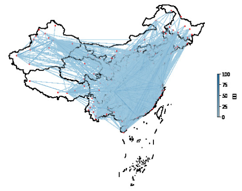
Identifying influential spreaders in complex networks is a crucial issue that can help control the propagation process in complex networks. An aviation network is a typical complex network, and accurately identifying the key city nodes in the aviation network can help us better prevent network attacks and control the spread of diseases. In this paper, a method for identifying key nodes in undirected weighted networks, called weighted Laplacian energy centrality, was proposed and applied to an aviation network constructed from real flight data. Based on the analysis of the topological structure of the network, the paper recognized critical cities in this network, then simulation experiments were conducted on key city nodes from the perspectives of network dynamics and robustness. The results indicated that, compared with other methods, weighted Laplacian energy centrality can identify the city nodes with the most spreading influence in the network. From the perspective of network robustness, the identified key nodes also have the characteristics of accurately and quickly destroying network robustness.
Citation: Shuying Zhao, Shaowei Sun. A study on centrality measures in weighted networks: A case of the aviation network[J]. AIMS Mathematics, 2024, 9(2): 3630-3645. doi: 10.3934/math.2024178
Identifying influential spreaders in complex networks is a crucial issue that can help control the propagation process in complex networks. An aviation network is a typical complex network, and accurately identifying the key city nodes in the aviation network can help us better prevent network attacks and control the spread of diseases. In this paper, a method for identifying key nodes in undirected weighted networks, called weighted Laplacian energy centrality, was proposed and applied to an aviation network constructed from real flight data. Based on the analysis of the topological structure of the network, the paper recognized critical cities in this network, then simulation experiments were conducted on key city nodes from the perspectives of network dynamics and robustness. The results indicated that, compared with other methods, weighted Laplacian energy centrality can identify the city nodes with the most spreading influence in the network. From the perspective of network robustness, the identified key nodes also have the characteristics of accurately and quickly destroying network robustness.

| [1] |
M. Ouyang, Z. Pan, L. Hong, L. Zhao, Correlation analysis of different vulnerability metrics on power grids, Physica A, 396 (2014), 204–211. https://doi.org/10.1016/j.physa.2013.10.041 doi: 10.1016/j.physa.2013.10.041

|
| [2] |
B. S. Kerner, Criticism of generally accepted fundamentals and methodologies of traffic and transportation theory: A brief review, Physica A, 391 (2013), 5261–5282. https://doi.org/10.1016/j.physa.2013.06.004 doi: 10.1016/j.physa.2013.06.004
|
| [3] |
D. Chen, H. Gao, L. Lü, T. Zhou, Identifying influential nodes in large-scale directed networks: The role of clustering, PLoS One, 8 (2013), e77455. https://doi.org/10.1371/journal.pone.0077455 doi: 10.1371/journal.pone.0077455
|
| [4] |
D. Chen, L. Lü, M. Shang, Y. Zhang, T. Zhou, Identifying influential nodes in complex networks, Physica A, 391 (2012), 1777–1887. https://doi.org/10.1016/j.physa.2011.09.017 doi: 10.1016/j.physa.2011.09.017
|
| [5] |
B. Michele, C. Davide, V. Simone, Efficiency of attack strategies on complex model and real-world networks, Physica A, 414 (2014), 174–180. https://doi.org/10.1016/j.physa.2014.06.079 doi: 10.1016/j.physa.2014.06.079
|
| [6] |
S. P. Borgatti, Identifying sets of key players in a social network, Comput. Math. Organ. Theory, 12 (2006), 21–34. https://doi.org/10.1007/s10588-006-7084-x doi: 10.1007/s10588-006-7084-x
|
| [7] |
T. Wen, D. Pelusi, Y. Deng, Vital spreaders identification in complex networks with multi-local dimension, Knowl. Based Syst., 195 (2020), 105717. https://doi.org/10.1016/j.knosys.2020.105717 doi: 10.1016/j.knosys.2020.105717
|
| [8] |
J. Zhao, Y. Song, F. Liu, Y. Deng, The identification of influential nodes based on structure similarity, Connect. Sci., 33 (2021), 201–218. https://doi.org/10.1080/09540091.2020.1806203 doi: 10.1080/09540091.2020.1806203
|
| [9] |
L. Freeman, Centrality in social networks conceptual clarification, Soc. Networks, 1 (1978), 215–239. https://doi.org/10.1016/0378-8733(78)90021-7 doi: 10.1016/0378-8733(78)90021-7
|
| [10] |
A. Barrat, M. Barthelemyt, R. Pastor-Satorrast, A. Vespignani, The architecture of complex weighted networks, PNAS, 101 (2004), 3747–3752. https://doi.org/10.1073/pnas.0400087101 doi: 10.1073/pnas.0400087101
|
| [11] | G. Sabidussi, The centrality index of a graph, Psychometrika, 31 (1966), 581–603. |
| [12] |
L. Freeman, A set of measures of centrality based upon betweenness, Sociometry, 40 (1977), 35–41. https://doi.org/10.2307/3033543 doi: 10.2307/3033543
|
| [13] |
T. Opsahl, F. Agneessens, J. Skvoretzc, Node centrality in weighted networks: Generalizing degree and shortest paths, Soc. Networks, 32 (2010), 245–251. https://doi.org/10.1016/j.socnet.2010.03.006 doi: 10.1016/j.socnet.2010.03.006
|
| [14] |
Y. Ma, Z. Cao, X. Qi, Quasi-Laplacian centrality: A new vertex centrality measurement based on Quasi-Laplacian energy of networks, Physica A, 527 (2019), 121130. https://doi.org/10.1016/j.physa.2019.121130 doi: 10.1016/j.physa.2019.121130
|
| [15] |
S. Zhao, S. Sun, Identification of node centrality based on Laplacian energy of networks, Physica A, 609 (2023), 128353. https://doi.org/10.1016/j.physa.2022.128353 doi: 10.1016/j.physa.2022.128353
|
| [16] |
S. Bansal, J. Sen, Network assessment of Tier-Ⅱ Indian cities airports in terms of type, accessibility, and connectivity, Transp. Policy, 124 (2022), 221–232. https://doi.org/10.1016/j.tranpol.2021.05.009 doi: 10.1016/j.tranpol.2021.05.009
|
| [17] |
R. W. Daniel, R. Soumen, M. D. S. Raissa, Resilience and rewiring of the passenger airline networks in the United States, Phys. Rev. E, 82 (2010), 056101. https://doi.org/10.1103/PhysRevE.82.056101 doi: 10.1103/PhysRevE.82.056101
|
| [18] | A. Reggiani, S. Signoretti, P. Nijkamp, A. Cento, Network measures in civil air transport: A case study of lufthansa, 1 Eds., Berlin: Springer Press, 2009. https://doi.org/10.1007/978-3-540-68409-1-14 |
| [19] |
J. Shen, H. Zong, Identification of critical transportation cities in the multimodal transportation network of China, Physica A, 628 (2023), 129174. https://doi.org/10.1016/j.physa.2023.129174 doi: 10.1016/j.physa.2023.129174
|
| [20] | F. Gao, Y. Dang, Analysis on distribution property of an international air transport network, Sci. Sci. Manage. S. T., 7 (2009), 75–79. |
| [21] |
R. Guimera, L. Amaral, Modeling the world-wide airport network, Eur. Phys. J. B, 38 (2004), 381–385. https://doi.org/10.1140/epjb/e2004-00131-0 doi: 10.1140/epjb/e2004-00131-0
|
| [22] |
J. Hu, Y. Wang, X. He, Analysis and application of global aviation network based on complex network, Comput. Sci., 48 (2021), 321–325. https://doi.org/10.11896/jsjkx.200900112 doi: 10.11896/jsjkx.200900112
|
| [23] | W. Liu, M. Han, Z. Xie, Connectivity characteristics and community identification of worldcity network based on global airline, Econ. Geogr., 40 (2020), 34–40. |
| [24] |
O. Lordan, J. Sallan, P Simo, Robustness of the air transport network, Transp. Res. Part E, 68 (2014), 155–163. https://doi.org/10.1016/j.tre.2014.05.011 doi: 10.1016/j.tre.2014.05.011
|
| [25] |
H. Mo, F. Jin, Y. Liu, J. Wang, Network analysis on centrality of airport system, Sci. Geol. Sin., 30 (2010), 204–212. https://doi.org/10.13249/j.cnki.sgs.2010.02.204 doi: 10.13249/j.cnki.sgs.2010.02.204
|
| [26] |
J. Li, X. Wen, M. Wu, F. Liu, S. Li, Identification of key nodes and vital edges in aviation network based on minimum connected dominating set, Physica A, 87 (2020), 123340. https://doi.org/10.1016/j.physa.2019.123340 doi: 10.1016/j.physa.2019.123340
|
| [27] | X. Luo, J. Wen, J. Zhong, Structural characteristics and robustness analysis of state-owned airline networks, Aeronaut. Comput. Tech., 51 (2021), 55–59. |
| [28] |
D. J. Watts, S. H. Strogatz, Collective dynamics of 'small-world' networks, Nature, 393 (1998), 440–442. https://doi.org/10.1038/30918 doi: 10.1038/30918
|
| [29] | X. Feng, H. Jia, Aviation network robustness considering node failure and edge failure, J. Beijing Jiaotong Univ., 45 (2021), 84–92. |
| [30] |
M. E. J. Newman, Y. Liu, Scientific collaboration networks. Ⅱ. Shortest paths, weighted networks, and centrality, Phys. Rev. E, 64 (2001), 016132. https://doi.org/10.1103/PhysRevE.64.016132 doi: 10.1103/PhysRevE.64.016132
|
| [31] |
P. Bonacich, Power and centrality: A family of measures, Am. J. Sociol., 92 (1987), 1170–1182. https://doi.org/10.1086/228631 doi: 10.1086/228631
|
| [32] |
K. Dietz, Infectious diseases of humans: Dynamics and control, Ann. Inter. Med., 117 (1992), 179. https://doi.org/10.1016/0169-4758(92)90018-W doi: 10.1016/0169-4758(92)90018-W
|
| [33] |
V. Latora, M. Marchiori, Efficient behavior of small-world networks, Phys. Rev. Lett., 87 (2001), 198701. https://doi.org/10.1103/PhysRevLett.87.198701 doi: 10.1103/PhysRevLett.87.198701
|
| [34] |
C. Castellano, R. Pastor-Satorras, Thresholds for epidemic spreading in networks, Phys. Rev. Lett., 105 (2010), 218701. https://doi.org/10.1103/PhysRevLett.105.218701 doi: 10.1103/PhysRevLett.105.218701
|


Figures(4) / Tables(1)

Shuying Zhao, Shaowei Sun. A study on centrality measures in weighted networks: A case of the aviation network[J]. AIMS Mathematics, 2024, 9(2): 3630-3645. doi: 10.3934/math.2024178


 DownLoad: