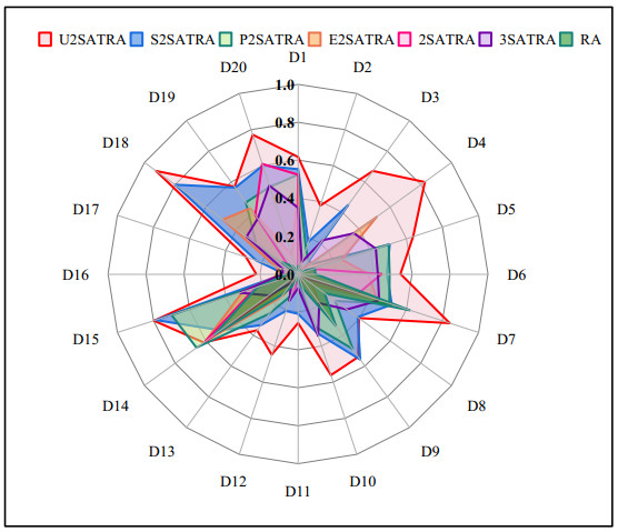
Evaluating behavioral patterns through logic mining within a given dataset has become a primary focus in current research. Unfortunately, there are several weaknesses in the research regarding the logic mining models, including an uncertainty of the attribute selected in the model, random distribution of negative literals in a logical structure, non-optimal computation of the best logic, and the generation of overfitting solutions. Motivated by these limitations, a novel logic mining model incorporating the mechanism to control the negative literal in the systematic Satisfiability, namely Weighted Systematic 2 Satisfiability in Discrete Hopfield Neural Network, is proposed as a logical structure to represent the behavior of the dataset. For the proposed logic mining models, we used ratio of r to control the distribution of the negative literals in the logical structures to prevent overfitting solutions and optimize synaptic weight values. A new computational approach of the best logic by considering both true and false classification values of the learning system was applied in this work to preserve the significant behavior of the dataset. Additionally, unsupervised learning techniques such as Topological Data Analysis were proposed to ensure the reliability of the selected attributes in the model. The comparative experiments of the logic mining models by utilizing 20 repository real-life datasets were conducted from repositories to assess their efficiency. Following the results, the proposed logic mining model dominated in all the metrics for the average rank. The average ranks for each metric were Accuracy (7.95), Sensitivity (7.55), Specificity (7.93), Negative Predictive Value (7.50), and Mathews Correlation Coefficient (7.85). Numerical results and in-depth analysis demonstrated that the proposed logic mining model consistently produced optimal induced logic that best represented the real-life dataset for all the performance metrics used in this study.
Citation: Nurul Atiqah Romli, Nur Fariha Syaqina Zulkepli, Mohd Shareduwan Mohd Kasihmuddin, Nur Ezlin Zamri, Nur 'Afifah Rusdi, Gaeithry Manoharam, Mohd. Asyraf Mansor, Siti Zulaikha Mohd Jamaludin, Amierah Abdul Malik. Unsupervised logic mining with a binary clonal selection algorithm in multi-unit discrete Hopfield neural networks via weighted systematic 2 satisfiability[J]. AIMS Mathematics, 2024, 9(8): 22321-22365. doi: 10.3934/math.20241087
Evaluating behavioral patterns through logic mining within a given dataset has become a primary focus in current research. Unfortunately, there are several weaknesses in the research regarding the logic mining models, including an uncertainty of the attribute selected in the model, random distribution of negative literals in a logical structure, non-optimal computation of the best logic, and the generation of overfitting solutions. Motivated by these limitations, a novel logic mining model incorporating the mechanism to control the negative literal in the systematic Satisfiability, namely Weighted Systematic 2 Satisfiability in Discrete Hopfield Neural Network, is proposed as a logical structure to represent the behavior of the dataset. For the proposed logic mining models, we used ratio of r to control the distribution of the negative literals in the logical structures to prevent overfitting solutions and optimize synaptic weight values. A new computational approach of the best logic by considering both true and false classification values of the learning system was applied in this work to preserve the significant behavior of the dataset. Additionally, unsupervised learning techniques such as Topological Data Analysis were proposed to ensure the reliability of the selected attributes in the model. The comparative experiments of the logic mining models by utilizing 20 repository real-life datasets were conducted from repositories to assess their efficiency. Following the results, the proposed logic mining model dominated in all the metrics for the average rank. The average ranks for each metric were Accuracy (7.95), Sensitivity (7.55), Specificity (7.93), Negative Predictive Value (7.50), and Mathews Correlation Coefficient (7.85). Numerical results and in-depth analysis demonstrated that the proposed logic mining model consistently produced optimal induced logic that best represented the real-life dataset for all the performance metrics used in this study.

| [1] |
J. J. Hopfield, D. W. Tank, "Neural" computation of decisions in optimization problems, Biol. Cybern., 52 (1985), 141–152. https://doi.org/10.1007/BF00339943 doi: 10.1007/BF00339943

|
| [2] |
W. A. T. W. Abdullah, Logic programming on a neural network, Int. J. Intell. Syst., 7 (1992), 513–519. https://doi.org/10.1002/int.4550070604 doi: 10.1002/int.4550070604
|
| [3] | M. S. M. Kasihmuddin, M. A. Mansor, S. Sathasivam, Hybrid genetic algorithm in the hopfield network for logic satisfiability problem, Pertanika J. Sci. Technol., 25 (2017). |
| [4] | M. A. Mansor, M. S. M. Kasihmuddin, S. Sathasivam, Artificial immune system paradigm in the hopfield network for 3-satisfiability problem, Pertanika J. Sci. Technol., 25 (2017). |
| [5] |
S. Sathasivam, M. A. Mansor, M. S. M. Kasihmuddin, H. Abubakar, Election algorithm for random k satisfiability in the hopfield neural network, Processes, 8 (2020), 568. https://doi.org/10.3390/PR8050568 doi: 10.3390/PR8050568
|
| [6] |
S. Sathasivam, M. A. Mansor, A. I. M. Ismail, S. Z. M. Jamaludin, M. S. M. Kasihmuddin, M. Mamat, Novel random k satisfiability for k ≤ 2 in hopfield neural network, Sains Malays., 49 (2020), 2847–2857. https://doi.org/10.17576/jsm-2020-4911-23 doi: 10.17576/jsm-2020-4911-23
|
| [7] |
S. A. Karim, N. E. Zamri, A. Alway, M. S. M. Kasihmuddin, A. I. M. Ismail, M. A. Mansor, et al., Random satisfiability: A higher-order logical approach in discrete hopfield neural network, IEEE Access, 9 (2021), 50831–50845. https://doi.org/10.1109/ACCESS.2021.3068998 doi: 10.1109/ACCESS.2021.3068998
|
| [8] |
Y. Guo, M. S. M. Kasihmuddin, Y. Gao, M. A. Mansor, H. A. Wahab, N. E. Zamri, et al., YRAN2SAT: A novel flexible random satisfiability logical rule in discrete hopfield neural network, Adv. Eng. Softw., 171 (2022), 103169. https://doi.org/10.1016/j.advengsoft.2022.103169 doi: 10.1016/j.advengsoft.2022.103169
|
| [9] |
N. E. Zamri, S. A. Azhar, S. S. M. Sidik, M. A. Mansor, M. S. M. Kasihmuddin, S. P. A. Pakruddin, et al., Multi-discrete genetic algorithm in hopfield neural network with weighted random k satisfiability, Neural Comput. Appl., 34 (2022) 19283–19311. https://doi.org/10.1007/s00521-022-07541-6 doi: 10.1007/s00521-022-07541-6
|
| [10] |
S. Sathasivam, W. A. T. Wan Abdullah, Logic mining in neural network: Reverse analysis method, Computing, 91 (2011), 119–133. https://doi.org/10.1007/s00607-010-0117-9 doi: 10.1007/s00607-010-0117-9
|
| [11] | L. C. Kho, M. S. M. Kasihmuddin, M. A. Mansor, S. Sathasivam, Logic mining in league of legends, Pertanika J. Sci. Technol., 28 (2020). |
| [12] |
N. E. Zamri, M. A. Mansor, M. S. M. Kasihmuddin, A. Alway, S. Z. M. Jamaludin, S. A. Alzaeemi, Amazon employees resources access data extraction via clonal selection algorithm and logic mining approach, Entropy, 22 (2020), 596. https://doi.org/10.3390/E22060596 doi: 10.3390/E22060596
|
| [13] |
S. Z. M. Jamaludin, M. S. M. Kasihmuddin, A. I. M. Ismail, M. A. Mansor, M. F. M. Basir, Energy based logic mining analysis with hopfield neural network for recruitment evaluation, Entropy, 23 (2021). https://doi.org/10.3390/e23010040 doi: 10.3390/e23010040
|
| [14] |
S. Z. M. Jamaludin, M. A. Mansor, A. Baharum, M. S. M. Kasihmuddin, H. A. Wahab, M. F. Marsani, Modified 2 satisfiability reverse analysis method via logical permutation operator, Comput. Mater. Contin., 74 (2023), 2853–2870. https://doi.org/10.32604/cmc.2023.032654 doi: 10.32604/cmc.2023.032654
|
| [15] |
M. S. M. Kasihmuddin, S. Z. M. Jamaludin, M. A. Mansor, H. A. Wahab, S. M. S. Ghadzi, Supervised learning perspective in logic mining, Mathematics, 10 (2022), 915. https://doi.org/10.3390/math10060915 doi: 10.3390/math10060915
|
| [16] |
S. Z. M. Jamaludin, N. A. Romli, M. S. M. Kasihmuddin, A. Baharum, M. A. Mansor, M. F. Marsani, Novel logic mining incorporating log linear approach, J. King Saud Univ.-Comput. Inf. Sci., 34 (2022), 9011–9027. https://doi.org/10.1016/j.jksuci.2022.08.026 doi: 10.1016/j.jksuci.2022.08.026
|
| [17] |
N. A. Rusdi, M. S. M. Kasihmuddin, N. A. Romli, G. Manoharam, M. A. Mansor, Multi-unit discrete hopfield neural network for higher order supervised learning through logic mining: Optimal performance design and attribute selection, J. King Saud Univ.–Com., 35 (2023), 101554. https://doi.org/10.1016/j.jksuci.2023.101554 doi: 10.1016/j.jksuci.2023.101554
|
| [18] |
G. Manoharam, M. S. M. Kasihmuddin, S. N. F. M. A. Antony, N. A. Romli, N. A. Rusdi, S. Abdeen, et al., Log-linear-based logic mining with multi-discrete hopfield neural network, Mathematics, 9 (2023), 2121. https://doi.org/10.3390/math11092121 doi: 10.3390/math11092121
|
| [19] |
A. Alway, N. E. Zamri, M. A. Mansor, M. S. M. Kasihmuddin, S. Z. M. Jamaludin, M. F. Marsani, A novel hybrid exhaustive search and data preparation technique with multi-objective discrete hopfield neural network, Decis. Anal., 9 (2023), 100354. https://doi.org/10.1016/j.dajour.2023.100354 doi: 10.1016/j.dajour.2023.100354
|
| [20] |
N. E. Zamri, M. A. Mansor, M. S. M. Kasihmuddin, S. S. Sidik, A. Alway, N. A. Romli, et al., A modified reverse-based analysis logic mining model with weighted random 2 satisfiability logic in discrete hopfield neural network and multi-objective training of modified niched genetic algorithm, Expert Syst. Appl., 240 (2024) 122307. 2024. https://doi.org/10.1016/j.eswa.2023.122307 doi: 10.1016/j.eswa.2023.122307
|
| [21] |
N. E. Zamri, S. A. Azhar, M. A. Mansor, A. Alway, M. S. M. Kasihmuddin, Weighted random k satisfiability for k = 1, 2 (r2SAT) in discrete hopfield neural network, Appl. Soft Comput., 126 (2022), 109312. https://doi.org/10.1016/j.asoc.2022.109312 doi: 10.1016/j.asoc.2022.109312
|
| [22] |
D. Bajusz, A. Rácz, K. Héberger, Why is Tanimoto index an appropriate choice for fingerprint-based similarity calculations? J. Cheminformatics, 7 (2015), 1–13. https://doi.org/10.1186/s13321-015-0069-3 doi: 10.1186/s13321-015-0069-3
|
| [23] | L. N. De Castro, F. J. von Zuben, The clonal selection algorithm with engineering applications, Gecco, 2000 (2000), 36–39. |
| [24] |
Y. Zhu, W. Li, T. Li, A hybrid artificial immune optimization for high-dimensional feature selection, Knowl.-Based Syst., 260 (2023), 11011. https://doi.org/10.1016/j.knosys.2022.110111 doi: 10.1016/j.knosys.2022.110111
|
| [25] | G. Singh, F. Mémoli, G. Carlsson, Topological methods for the analysis of high dimensional data sets and 3D object recognition, In: 4th symposium on point based graphics, PBG@Eurographics 2007, 2007. |
| [26] |
A. D. Smith, P. Dłotko, V. M. Zavala, Topological data analysis: Concepts, computation, and applications in chemical engineering, Comput. Chem. Eng., 146 (2021), 107202. https://doi.org/10.1016/j.compchemeng.2020.107202 doi: 10.1016/j.compchemeng.2020.107202
|
| [27] |
Y. Chen, I. Volic, Topological data analysis model for the spread of the coronavirus, Plos One, 16 (2021), e0255584. https://doi.org/10.1371/journal.pone.0255584 doi: 10.1371/journal.pone.0255584
|
| [28] |
O. Kwon, J. M. Sim, Effects of data set features on the performances of classification algorithms, Expert Syst. Appl., 40 (2013), 1847–1857. https://doi.org/10.1016/j.eswa.2012.09.017 doi: 10.1016/j.eswa.2012.09.017
|
| [29] |
J. Dou, Y. Song, G. Wei, Y. Zhang, Fuzzy information decomposition incorporated and weighted Relief-F feature selection: When imbalanced data meet incompletion, Inf. Sci., 584 (2022), 417–432. https://doi.org/10.1016/j.ins.2021.10.057 doi: 10.1016/j.ins.2021.10.057
|
| [30] |
K. Jha, S. Saha, Incorporation of multimodal multiobjective optimization in designing a filter based feature selection technique, Appl. Soft Comput., 98 (2021), 106823. https://doi.org/10.1016/j.asoc.2020.106823 doi: 10.1016/j.asoc.2020.106823
|
| [31] |
S. Sen, A. V. Deokar, Toward understanding variations in price and billing in US healthcare services: A predictive analytics approach, Expert Syst. Appl., 209 (2022), 118241. https://doi.org/10.1016/j.eswa.2022.118241 doi: 10.1016/j.eswa.2022.118241
|
| [32] |
S. Hasija, P. Akash, M. B. Hemanth, A. Kumar, S. Sharma, A novel approach for detection of COVID-19 and Pneumonia using only binary classification from chest CT-scans, Neurosci. Inform., 2 (2022), 100069. https://doi.org/10.1016/j.neuri.2022.100069 doi: 10.1016/j.neuri.2022.100069
|
| [33] |
A. Luque, A. Carrasco, A. Martín, A. de las Heras, The impact of class imbalance in classification performance metrics based on the binary confusion matrix, Pattern Recognit., 91 (2019), 216–231. https://doi.org/10.1016/j.patcog.2019.02.023 doi: 10.1016/j.patcog.2019.02.023
|
| [34] |
F. Amin, M. Mahmoud, Confusion matrix in binary classification problems: A step-by-step tutorial, J. Eng. Res., 6 (2022). https://doi.org/10.21608/erjeng.2022.274526 doi: 10.21608/erjeng.2022.274526
|
| [35] |
M. Ohsaki, P. Wang, K. Matsuda, S. Katagiri, H. Watanabe, A. Ralescu, Confusion-matrix-based kernel logistic regression for imbalanced data classification, IEEE Trans. Knowl. Data Eng., 29 (2017), 1806–1819. https://doi.org/10.1109/TKDE.2017.2682249 doi: 10.1109/TKDE.2017.2682249
|
| [36] |
J. Gorodkin, Comparing two K-category assignments by a K-category correlation coefficient, Comput. Biol. Chem., 28 (2004), 367–374. https://doi.org/10.1016/j.compbiolchem.2004.09.006 doi: 10.1016/j.compbiolchem.2004.09.006
|
| [37] |
D. Chicco, G. Jurman, The advantages of the Matthews correlation coefficient (MCC) over F1 score and accuracy in binary classification evaluation, BMC Genomics, 21 (2020), 1–13. https://doi.org/10.1186/s12864-019-6413-7 doi: 10.1186/s12864-019-6413-7
|
| [38] |
V. Someetheram, M. F. Marsani, M. S. M. Kasihmuddin, N. E. Zamri, S. S. M. Sidik, S. Z. M. Jamaludin, et al., Random maximum 2 satisfiability logic in discrete hopfield neural network incorporating improved election algorithm, Mathematics, 10 (2022), 4734. https://doi.org/10.3390/math10244734 doi: 10.3390/math10244734
|
| [39] |
S. Abdeen, M. S. M. Kasihmuddin, N. E. Zamri, G. Manoharam, M. A. Mansor, N. Alshehri, S-type random k satisfiability logic in discrete hopfield neural network using probability distribution: Performance optimization and analysis, Mathematics, 11 (2023), 984. https://doi.org/10.3390/math11040984 doi: 10.3390/math11040984
|
| [40] |
A. Alway, N. E. Zamri, S. A. Karim, M. A. Mansor, M. S. M. Kasihmuddin, M. M. Bazuhair, Major 2 satisfiability logic in discrete hopfield neural network, Int. J. Comput. Math., 99 (2022), 924–948. https://doi.org/10.1080/00207160.2021.1939870 doi: 10.1080/00207160.2021.1939870
|
| [41] |
C. Iwendi, K. Mahboob, Z. Khalid, A. R. Javed, M. Rizwan, U. Ghosh, Classification of COVID-19 individuals using adaptive neuro-fuzzy inference system, Multimedia Syst., 2022, 1–15. https://doi.org/10.1007/s00530-021-00774-w doi: 10.1007/s00530-021-00774-w
|
| [42] |
M. Herland, R. A. Bauder, T. M. Khoshgoftaar, The effects of class rarity on the evaluation of supervised healthcare fraud detection models, J. Big Data, 6 (2019), 1–33. https://doi.org/10.1186/s40537-019-0181-8 doi: 10.1186/s40537-019-0181-8
|
| [43] |
M. Noureddin, E. Truong, J. A. Gornbein, R. Saouaf, M. Guindi, T. Todo, et al., MRI-based (MAST) score accurately identifies patients with NASH and significant fibrosis, J. Hepatol., 76 (2022), 781–787. https://doi.org/10.1016/j.jhep.2021.11.012 doi: 10.1016/j.jhep.2021.11.012
|
| [44] |
P. Ong, Z. Zainuddin, Optimizing wavelet neural networks using modified cuckoo search for multi-step ahead chaotic time series prediction, Appl. Soft Compt., 80 (2019), 374–386. https://doi.org/10.1016/j.asoc.2019.04.016 doi: 10.1016/j.asoc.2019.04.016
|
| [45] |
H. L. Li, J. Cao, C. Hu, H. Jiang, A. Alsaedi, Synchronization analysis of nabla fractional-order fuzzy neural networks with time delays via nonlinear feedback control, Fuzzy Set. Syst., 475 (2024), 108750. https://doi.org/10.1016/j.fss.2023.108750 doi: 10.1016/j.fss.2023.108750
|
| [46] |
H. L. Li, J. Cao, C. Hu, L. Zhang, H. Jiang, Adaptive control-based synchronization of discrete-time fractional-order fuzzy neural networks with time-varying delays, Neural Netw., 168 (2023), 59–73. https://doi.org/10.1016/j.neunet.2023.09.019 doi: 10.1016/j.neunet.2023.09.019
|
| [47] |
J. Cao, K. Udhayakumar, R. Rakkiyappan, X. Li, J. Lu, A comprehensive review of continuous-/discontinuous-time fractional-order multidimensional neural networks, IEEE Trans. Neural Netw. Learn. Syst., 34 (2021), 5476–5496. https://doi.org/10.1109/TNNLS.2021.3129829 doi: 10.1109/TNNLS.2021.3129829
|
Figures(9) / Tables(14)

Nurul Atiqah Romli, Nur Fariha Syaqina Zulkepli, Mohd Shareduwan Mohd Kasihmuddin, Nur Ezlin Zamri, Nur 'Afifah Rusdi, Gaeithry Manoharam, Mohd. Asyraf Mansor, Siti Zulaikha Mohd Jamaludin, Amierah Abdul Malik. Unsupervised logic mining with a binary clonal selection algorithm in multi-unit discrete Hopfield neural networks via weighted systematic 2 satisfiability[J]. AIMS Mathematics, 2024, 9(8): 22321-22365. doi: 10.3934/math.20241087


 DownLoad: