A new approach of overlapping generation model via fixed point technique

Abdelkader Belhenniche; Monica-Felicia Bota; Liliana Guran; Abdelkader Belhenniche; Monica-Felicia Bota; Liliana Guran

doi:10.3934/math.2024057

AIMS Mathematics

2024, Volume 9, Issue 1: 1166-1179. doi: 10.3934/math.2024057

Previous Article Next Article

Research article

A new approach of overlapping generation model via fixed point technique

1.
Research Center for Systems and Technologies (SYSTEC), ARISE, Faculty of Engineering, University of Porto, Rua Dr. Roberto Frias s/n, office i102, 4200-465 Porto, Portugal
2.
Laboratoire d'Etudes Pratiques en Sciences de Gestion et Sciences Commerciales, Ecole Supérieure de Commerce, 42003 Kolea, Tipaza, Algérie
3.
Department of Mathematics, Babeş-Bolyai University, M. Kogălniceanu Street, No. 1, 400084, Cluj-Napoca, Romania
4.
Department of Hospitality Services, Babeş-Bolyai University, Horea Street, No. 7, 400174, Cluj-Napoca, Romania

Received: 17 August 2023 Revised: 26 October 2023 Accepted: 07 November 2023 Published: 06 December 2023
MSC : 45G15, 47H10

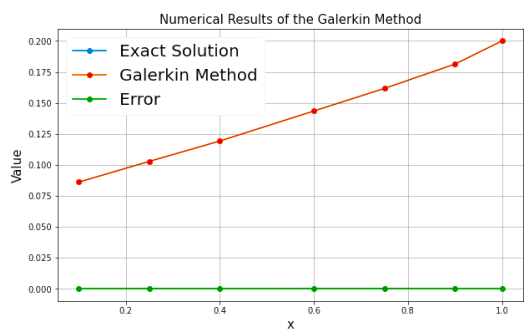
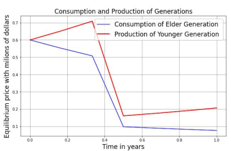
This article explored a specific variant of the overlapping generation model using a nonlinear Fredholm integral equation. We considered assumptions related to the Ćirić operator, offering a new perspective compared to existing research. To solve the equation, we employed the Galerkin method, which approximates it as a finite system of equations. By combining these approaches, we conducted a comprehensive analysis of the model, providing insights into its dynamics and potential applications.
- overlapping generation model,
- nonlinear Fredholm equation,
- Ćirić contractive maps,
- Galerkin method,
- fixed point theory
Citation: Abdelkader Belhenniche, Monica-Felicia Bota, Liliana Guran. A new approach of overlapping generation model via fixed point technique[J]. AIMS Mathematics, 2024, 9(1): 1166-1179. doi: 10.3934/math.2024057

Related Papers:

Abstract

This article explored a specific variant of the overlapping generation model using a nonlinear Fredholm integral equation. We considered assumptions related to the Ćirić operator, offering a new perspective compared to existing research. To solve the equation, we employed the Galerkin method, which approximates it as a finite system of equations. By combining these approaches, we conducted a comprehensive analysis of the model, providing insights into its dynamics and potential applications.

References

[1]	P. A. Diamond, National debt in a neoclassical growth model, Am. Econ. Rev., 55 (1965), 1126–1150. https://doi.org/10.1090/S0894-0347-1992-1124979-1 doi: 10.1090/S0894-0347-1992-1124979-1
[2]	C. Edmond, An integral equation representation for overlapping generations in continuous time, J. Econ. Theory, 134 (2008), 596–609. https://doi.org/10.1016/j.jet.2008.03.006 doi: 10.1016/j.jet.2008.03.006
[3]	P. Weil, Overlapping families of infinitely-lived agents, J. Public Econ., 27 (1983), 183–198. https://doi.org/10.1016/0047-2727(89)90024-8 doi: 10.1016/0047-2727(89)90024-8
[4]	I. Fredholm, Sur une classe d'équations fonctionnelles, Acta Math., 19 (1903), 365–390.
[5]	Z. Zou, R. Guo, The Riemann-Hilbert approach for the higher-order Gerdjikov-Ivanov equation, soliton interactions and position shift, Commun. Nonlinear Sci. Numer. Simulat., 124 (2023), 107316. https://doi.org/10.1016/j.cnsns.2023.107316 doi: 10.1016/j.cnsns.2023.107316
[6]	S. Shen, Z. Yang, X. Li, S. Zhang, Periodic propagation of complex-valued hyperbolic-cosine-Gaussian solitons and breathers with complicated light field structure in strongly nonlocal nonlinear media, Commun. Nonlinear Sci. Numer. Simulat., 103 (2021), 106005. https://doi.org/10.1016/j.cnsns.2021.106005 doi: 10.1016/j.cnsns.2021.106005
[7]	X. Li, R. Guo, Interactions of localized wave structures on periodic backgrounds for the coupled Lakshmanan-Porsezian-Daniel equations in birefringent optical fibers, Ann. Phys., 535 (2023), 2200472. https://doi.org/10.1002/andp.202200472 doi: 10.1002/andp.202200472
[8]	B. G. Galerkin, On electrical circuits for the approximate solution of the Laplace equation, Vestnik Inzh., 19 (1915), 897–908.
[9]	W. Hackbusch, S. A. Sauter, On the efficient use of the Galerkin-method to solve Fredholm integral equations, Appl. Math., 38 (1993), 301–322.
[10]	Z. Chen, Y. Xu, The Petrov-Galerkin and Iterated Petrov-Galerkin methods for second-kind integral equations, SIAM J. Numer., 35 (1998), 406–434. https://doi.org/10.1137/S0036142996297217 doi: 10.1137/S0036142996297217
[11]	S. Banach, Sur les opérations dans les ensembles abstraits et leur application aux équations intégrales, SIAM J. Numer., 26 (1922), 133–181.
[12]	L. B. Ćirić, A generalization of Banach's contraction principle, Proc. Am. Math. Soc, 45 (1974), 267–273.
[13]	L. B. Ćirić, Generalized contractions and fixed-point theorems, Publ. Inst. Math. Beograd, 26 (1971), 19–26.
[14]	L. B. Ćirić, Fixed-point theorems for multi-valued contractions in complete metric spaces, J. Math. Anal. Appl., 348 (2008), 499–507. https://doi.org/10.1016/j.jmaa.2008.07.062 doi: 10.1016/j.jmaa.2008.07.062

Reader Comments

Your name:*

Email:*
© 2024 the Author(s), licensee AIMS Press. This is an open access article distributed under the terms of the Creative Commons Attribution License (http://creativecommons.org/licenses/by/4.0)