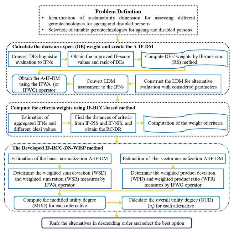
This study aims to introduce a decision-making framework for prioritizing gerontechnologies (GTs) for aging persons and people with disability under an intuitionistic fuzzy set (IFS) context. First, the intuitionistic fuzzy (IF)-divergence measure and its properties are developed to obtain the criteria weight. Second, a new exponential function-based score function and its properties for the IFS are introduced to order the different IFSs. Third, an IF-relative closeness coefficient (RCC)-based method is proposed to determine the criteria weights. Fourth, the double normalization (DN) procedure-based weighted integrated sum product (WISP) approach is introduced under the IFSs. To demonstrate the applicability and usefulness of the proposed IF-RCC-DN-WISP model, a case study that involves ranking the different GTs for aging persons and people with disability is conducted from an IF perspective. The results of the developed model show that mobility is the most appropriate gerontechnology for aging persons and people with disability. A comparison with different models is also performed to prove the superiority of the obtained results. The comparative study shows how the developed model outperforms the other extant models, as it can offer more sensible outcomes. Therefore, it is more suitable and efficient for expressing uncertain information when treating practical decision-making problems.
Citation: Ibrahim M. Hezam, Pratibha Rani, Arunodaya Raj Mishra, Ahmad M. Alshamrani. A combined intuitionistic fuzzy closeness coefficient and a double normalization-based WISP method to solve the gerontechnology selection problem for aging persons and people with disability[J]. AIMS Mathematics, 2023, 8(6): 13680-13705. doi: 10.3934/math.2023695
This study aims to introduce a decision-making framework for prioritizing gerontechnologies (GTs) for aging persons and people with disability under an intuitionistic fuzzy set (IFS) context. First, the intuitionistic fuzzy (IF)-divergence measure and its properties are developed to obtain the criteria weight. Second, a new exponential function-based score function and its properties for the IFS are introduced to order the different IFSs. Third, an IF-relative closeness coefficient (RCC)-based method is proposed to determine the criteria weights. Fourth, the double normalization (DN) procedure-based weighted integrated sum product (WISP) approach is introduced under the IFSs. To demonstrate the applicability and usefulness of the proposed IF-RCC-DN-WISP model, a case study that involves ranking the different GTs for aging persons and people with disability is conducted from an IF perspective. The results of the developed model show that mobility is the most appropriate gerontechnology for aging persons and people with disability. A comparison with different models is also performed to prove the superiority of the obtained results. The comparative study shows how the developed model outperforms the other extant models, as it can offer more sensible outcomes. Therefore, it is more suitable and efficient for expressing uncertain information when treating practical decision-making problems.

| [1] | F. Özsungur, Gerontechnological factors affecting successful aging of elderly, Aging Male, 23 (2020), 520–532. |
| [2] |
M. Haufe, S. T. M. Peek, K. G. Luijkx, Matching gerontechnologies to independent-living seniors' individual needs: Development of the GTM tool, BMC Health Serv. Res., 19 (2019), 1–13. https://doi.org/10.1186/s12913-018-3848-5 doi: 10.1186/s12913-018-3848-5

|
| [3] | F. Noublanche, C. Jaglin-Grimonprez, G. Sacco, N. Lerolle, P. Allain, C. Annweiler, The development of gerontechnology for hospitalized frail elderly people: The ALLEGRO hospital-based geriatric living lab, Maturitas, 125 (2019), 17–19. |
| [4] |
K. Halicka, D. Kacprzak, Linear ordering of selected gerontechnologies using selected MCGDM methods, Technol. Econ. Dev. Econ., 27 (2021), 921–947. https://doi.org/10.3846/tede.2021.15000 doi: 10.3846/tede.2021.15000
|
| [5] |
K. Halicka, Gerontechnology-the assessment of one selected technology improving the quality of life of older adults, Eng. Manag. Prod. Serv., 11 (2019), 43–51. https://doi.org/10.2478/emj-2019-0010 doi: 10.2478/emj-2019-0010
|
| [6] |
N. Rahmawati, B. C. Jiang, Develop a bedroom design guideline for progressive ageing residence: A case study of Indonesian older adults, Gerontechnology, 18 (2019), 180–192. https://doi.org/10.4017/gt.2019.18.3.005.00 doi: 10.4017/gt.2019.18.3.005.00
|
| [7] |
C. Namanee, N. Tuaycharoen, Task lighting for Thai older adults: Study of the visual performance of lighting effect characteristics, Gerontechnology, 18 (2019), 215–222. https://doi.org/10.4017/gt.2019.18.4.003.00 doi: 10.4017/gt.2019.18.4.003.00
|
| [8] |
L. A. Zadeh, Fuzzy sets, Inf. Control, 8 (1965), 338–353. https://doi.org/10.1016/S0019-9958(65)90241-X doi: 10.1016/S0019-9958(65)90241-X
|
| [9] |
A. Blagojević, S. Vesković, S. Kasalica, A. Gojić, A. Allamani, The application of the fuzzy AHP and DEA for measuring the efficiency of freight transport railway undertakings, Oper. Res. Eng. Sci. Theory Appl., 3 (2020), 1–23. https://doi.org/10.31181/oresta2003001b doi: 10.31181/oresta2003001b
|
| [10] |
S. Mustafa, A. A. Bajwa, S. Iqbal, A new fuzzy grach model to forecast stock market technical analysis, Oper. Res. Eng. Sci. Theory Appl., 5 (2022), 185–204. https://doi.org/10.31181/oresta040422196m doi: 10.31181/oresta040422196m
|
| [11] |
P. Rani, A. R. Mishra, A. Mardani, F. Cavallaro, M. Alrasheedi, A. Alrashidi, A novel approach to extended fuzzy TOPSIS based on new divergence measures for renewable energy sources selection, J. Clean. Prod., 257 (2020), 120352. https://doi.org/10.1016/j.jclepro.2020.120352 doi: 10.1016/j.jclepro.2020.120352
|
| [12] |
V. L. G. Nayagam, P. Dhanasekaran, S. Jeevaraj, A complete ranking of incomplete trapezoidal information, J. Intell. Fuzzy Syst., 30 (2016), 3209–3225. https://doi.org/10.3233/IFS-152064 doi: 10.3233/IFS-152064
|
| [13] |
V. L. G. Nayagam, S. Jeevaraj, G. Sivaraman, Ranking of incomplete trapezoidal information, Soft Comput., 21 (2017), 7125–7140. https://doi.org/10.1007/s00500-016-2256-1 doi: 10.1007/s00500-016-2256-1
|
| [14] |
S. Jeevaraj, A note on multi-criteria decision-making using a complete ranking of generalized trapezoidal fuzzy numbers, Soft Comput., 26 (2022), 11225–11230. https://doi.org/10.1007/s00500-022-07467-0 doi: 10.1007/s00500-022-07467-0
|
| [15] |
K. T. Atanassov, Intuitionistic fuzzy sets, Fuzzy Sets Syst., 20 (1986), 87–96. https://doi.org/10.1016/S0165-0114(86)80034-3 doi: 10.1016/S0165-0114(86)80034-3
|
| [16] |
J. Yuan, X. Luo, Approach for multi-attribute decision making based on novel intuitionistic fuzzy entropy and evidential reasoning, Comput. Ind. Eng., 135 (2019), 643–654. https://doi.org/10.1016/j.cie.2019.06.031 doi: 10.1016/j.cie.2019.06.031
|
| [17] |
B. Yan, Y. Rong, L. Yu, Y. Huang, A hybrid intuitionistic fuzzy group decision framework and its application in urban rail transit system selection, Mathematics, 10 (2022), 2133. https://doi.org/10.3390/math10122133 doi: 10.3390/math10122133
|
| [18] |
M. Rasoulzadeh, S. A. Edalatpanah, M. Fallah, S. E. Najafi, A multi-objective approach based on Markowitz and DEA cross-efficiency models for the intuitionistic fuzzy portfolio selection problem, Decis. Mak. Appl. Manag. Eng., 5 (2022), 241–259. https://doi.org/10.31181/dmame0324062022e doi: 10.31181/dmame0324062022e
|
| [19] |
D. K. Tripathi, S. K. Nigam, P. Rani, A. R. Shah, New intuitionistic fuzzy parametric divergence measures and score function-based CoCoSo method for decision-making problems, Decis. Mak. Appl. Manag. Eng., 2022. https://doi.org/10.31181/dmame0318102022t doi: 10.31181/dmame0318102022t
|
| [20] |
I. Montes, N. R. Pal, S. Montes, Entropy measures for Atanassov intuitionistic fuzzy sets based on divergence, Soft Comput., 22 (2018), 5051–5071. https://doi.org/10.1007/s00500-018-3318-3 doi: 10.1007/s00500-018-3318-3
|
| [21] |
L. Zeng, H. Ren, T. Yang, N. Xiong, An intelligent expert combination weighting scheme for group decision making in railway reconstruction, Mathematics, 10 (2022), 549. https://doi.org/10.3390/math10040549 doi: 10.3390/math10040549
|
| [22] |
S. Jeevaraj, Similarity measure on interval valued intuitionistic fuzzy numbers based on non-hesitance score and its application to pattern recognition, Comput. Appl. Math., 39 (2020), 212. https://doi.org/10.1007/s40314-020-01250-3 doi: 10.1007/s40314-020-01250-3
|
| [23] |
S. Jeevaraj, R. Rajesh, V. L. G. Nayagam, A complete ranking of trapezoidal-valued intuitionistic fuzzy number: An application in evaluating social sustainability, Neural Comput. Appl., 35 (2023), 5939–5962. https://doi.org/10.1007/s00521-022-07983-y doi: 10.1007/s00521-022-07983-y
|
| [24] |
S. Jeevaraj, P. Gatiyala, S. H. Hashemkhani, Trapezoidal intuitionistic fuzzy power Heronian aggregation operator and its applications to multiple-attribute group decision-making, Axioms, 11 (2022), 588. https://doi.org/10.3390/axioms11110588 doi: 10.3390/axioms11110588
|
| [25] |
R. T. Ngan, M. Ali, L. H. Son, δ-equality of intuitionistic fuzzy sets: A new proximity measure and applications in medical diagnosis, Appl. Intell., 48 (2018), 499–525. https://doi.org/10.1007/s10489-017-0986-0 doi: 10.1007/s10489-017-0986-0
|
| [26] |
J. S. Chai, G. Selvachandran, F. Smarandache, V. C. Gerogiannis, L. H. Son, Q. T. Bui, et al., New similarity measures for single-valued neutrosophic sets with applications in pattern recognition and medical diagnosis problems, Complex Intell. Syst., 7 (2021), 703–723. https://doi.org/10.1007/s40747-020-00220-w doi: 10.1007/s40747-020-00220-w
|
| [27] |
Q. T. Bui, M. P. Ngo, V. Snasel, W. Pedrycz, B. Vo, Information measures based on similarity under neutrosophic fuzzy environment and multi-criteria decision problems, Eng. Appl. Artif. Intell., 122 (2023), 106026. https://doi.org/10.1016/j.engappai.2023.106026 doi: 10.1016/j.engappai.2023.106026
|
| [28] |
A. R. Mishra, P. Rani, F. Cavallaro, I. M. Hezam, An IVIF-distance measure and relative closeness coefficient-based model for assessing the sustainable development barriers to biofuel enterprises in India, Sustainability, 15 (2023), 4354. https://doi.org/10.3390/su15054354 doi: 10.3390/su15054354
|
| [29] |
A. R. Mishra, P. Rani, F. Cavallaro, I. M. Hezam, J. Lakshmi, An integrated intuitionistic fuzzy closeness coefficient-based OCRA method for sustainable urban transportation options selection, Axioms, 12 (2023), 144. https://doi.org/10.3390/axioms12020144 doi: 10.3390/axioms12020144
|
| [30] |
I. K. Vlachos, G. D. Sergiadis, Intuitionistic fuzzy information-Application to pattern recognition, Pattern Recognit. Lett., 28 (2007), 197–206. https://doi.org/10.1016/j.patrec.2006.07.004 doi: 10.1016/j.patrec.2006.07.004
|
| [31] |
I. Montes, N. R. Pal, V. Janiš, S. Montes, Divergence measures for intuitionistic fuzzy sets, IEEE Trans. Fuzzy Syst., 23 (2015), 444–456. https://doi.org/10.1109/TFUZZ.2014.2315654 doi: 10.1109/TFUZZ.2014.2315654
|
| [32] |
R. Joshi, S. Kumar, A dissimilarity Jensen-Shannon divergence measure for intuitionistic fuzzy sets, Int. J. Intell. Syst., 33 (2018), 2216–2235. https://doi.org/10.1002/int.22026 doi: 10.1002/int.22026
|
| [33] |
R. Verma, On intuitionistic fuzzy order-α divergence and entropy measures with MABAC method for multiple attribute group decision-making, J. Intell. Fuzzy Syst., 40 (2021), 1191–1217. https://doi.org/10.3233/JIFS-201540 doi: 10.3233/JIFS-201540
|
| [34] |
A. R. Mishra, A. Mardani, P. Rani, H. Kamyab, M. Alrasheedi, A new intuitionistic fuzzy combinative distance-based assessment framework to assess low-carbon sustainable suppliers in the maritime sector, Energy, 237 (2021), 121500. https://doi.org/10.1016/j.energy.2021.121500 doi: 10.1016/j.energy.2021.121500
|
| [35] |
D. K. Tripathi, S. K. Nigam, A. R. Mishra, A. R. Shah, A novel intuitionistic fuzzy distance measure-SWARA-COPRAS method for multi-criteria food waste treatment technology selection, Oper. Res. Eng. Sci. Theory Appl., 5 (2022). https://doi.org/10.31181/oresta111022106t doi: 10.31181/oresta111022106t
|
| [36] |
D. Stanujkic, G. Popovic, D. Karabasevic, I. Meidute-Kavaliauskiene, A. Ulutas, An integrated simple weighted sum product method—WISP, IEEE Trans. Eng. Manag., 70 (2021), 1933–1944. https://doi.org/10.1109/tem.2021.3075783 doi: 10.1109/tem.2021.3075783
|
| [37] |
D. Karabasevic, A. Ulutas, D. Stanujkic, M. Saracevic, G. Popovic, A new fuzzy extension of the simple WISP method, Axioms, 11 (2021), 332. https://doi.org/10.3390/axioms11070332 doi: 10.3390/axioms11070332
|
| [38] |
E. K. Zavadskas, D. Stanujkic, Z. Turskis, D. Karabasevic, An intuitionistic extension of the simple WISP method, Entropy, 24 (2022), 218. https://doi.org/10.3390/e24020218 doi: 10.3390/e24020218
|
| [39] |
D. Stanujkic, D. Karabasevic, G. Popovic, F. Smarandache, P. S. Stanimirović, M. Saračević, et al., A single valued neutrosophic extension of the simple WISP method, Informatica, 33 (2022), 635–651. https://doi.org/10.15388/22-INFOR483 doi: 10.15388/22-INFOR483
|
| [40] |
M. Deveci, A. R. Mishra, I. Gokasar, P. Rani, D. Pamucar, E. Ozcan, A decision support system for assessing and prioritizing sustainable urban transportation in metaverse, IEEE Trans. Fuzzy Syst., 31 (2023), 475–484. https://doi.org/10.1109/TFUZZ.2022.3190613 doi: 10.1109/TFUZZ.2022.3190613
|
| [41] |
Z. S. Xu, Intuitionistic fuzzy aggregation operators, IEEE Trans. Fuzzy Syst., 15 (2007), 1179–1187. https://doi.org/10.1109/TFUZZ.2006.890678 doi: 10.1109/TFUZZ.2006.890678
|
| [42] |
G. L. Xu, S. P. Wan, X. L. Xie, A selection method based on MAGDM with interval-valued intuitionistic fuzzy sets, Math. Probl. Eng., 2015 (2015), 1–13. https://doi.org/10.1155/2015/791204 doi: 10.1155/2015/791204
|
| [43] |
I. M. Hezam, A. R. Mishra, P. Rani, F. Cavallaro, A. Saha, J. Ali, et al., A hybrid intuitionistic fuzzy-MEREC-RS-DNMA method for assessing the alternative fuel vehicles with sustainability perspectives, Sustainability, 14 (2022), 5463. https://doi.org/10.3390/su14095463 doi: 10.3390/su14095463
|
| [44] | D. B. Ross, M. Eleno-Orama, E. V. Salah, The aging and technological society: Learning our way through the decades, In: Handbook of Research on Human Development in the Digital Age, IGI Global, 2018. https://doi.org/10.4018/978-1-5225-2838-8.ch010 |
| [45] | P. Sale, Gerontechnology, domotics, and robotics, In: Practical Issues in Geriatrics, Rehabilitation Medicine for Elderly Patients, Springer, 2018. https://doi.org/10.1007/978-3-319-57406-6_19 |
| [46] | T. Jansson, T. Kupiainen, Aged people's experiences of gerontechnology used at home, A narrative literature review, 2017. Available from: https://www.theseus.fi/bitstream/handle/10024/129279/Jansson_Kupiainen_ONT_21.4.17.pdf?sequence = 1 & isAllowed = y. |
| [47] | R. R. McWhorter, J. A. Delello, S. Gipson, B. Mastel-Smith, K. Caruso, Do loneliness and social connectedness improve in older adults through mobile technology? In: Disruptive and Emerging Technology Trends across Education and the Workplace, IGI Global, 2020,221–242. https://doi.org/10.4018/978-1-7998-2914-0.ch009 |
| [48] |
J. Nazarko, J. Ejdys, K. Halicka, A. Magruk, L. Nazarko, A. Skorek, Application of enhanced SWOT analysis in the future-oriented public management of technology, Procedia Eng., 182 (2017), 482–490. https://doi.org/10.1016/j.proeng.2017.03.140 doi: 10.1016/j.proeng.2017.03.140
|
| [49] |
R. Kumari, A. R. Mishra, Multi-criteria COPRAS method based on parametric measures for intuitionistic fuzzy sets: Application of green supplier selection, IJS-T. Elec. Eng., 44 (2020), 1645–1662. https://doi.org/10.1007/s40998-020-00312-w doi: 10.1007/s40998-020-00312-w
|
| [50] |
A. R. Mishra, A. Chandel, P. Saeidi, Low-carbon tourism strategy evaluation and selection using interval-valued intuitionistic fuzzy additive ratio assessment approach based on similarity measures, Environ. Dev. Sustain., 24 (2022), 7236–7282. https://doi.org/10.1007/s10668-021-01746-w doi: 10.1007/s10668-021-01746-w
|
| [51] |
P. Rani, A. R. Mishra, M. D. Ansari, A. Ali, Assessment of performance of telecom service providers using intuitionistic fuzzy grey relational analysis framework (IF-GRA), Soft Comput., 25 (2021), 1983–1993. https://doi.org/10.1007/s00500-020-05269-w doi: 10.1007/s00500-020-05269-w
|
| [52] | H. Gitinavard, M. A. Shirazi, An extended intuitionistic fuzzy modified group complex proportional assessment approach, J. Ind. Syst. Eng., 11 (2018), 229–246. |
| [53] |
A. R. Mishra, R. K. Singh, D. Motwani, Multi-criteria assessment of cellular mobile telephone service providers using intuitionistic fuzzy WASPAS method with similarity measures, Granul. Comput., 4 (2019), 511–529. https://doi.org/10.1007/s41066-018-0114-5 doi: 10.1007/s41066-018-0114-5
|
| [54] |
A. R. Mishra, P. Rani, F. Cavallaro, I. M. Hezam, Intuitionistic fuzzy fairly operators and additive ratio assessment-based integrated model for selecting the optimal sustainable industrial building options, Sci. Rep., 13 (2023), 5055. https://doi.org/10.1038/s41598-023-31843-x doi: 10.1038/s41598-023-31843-x
|
| [55] |
I. M. Hezam, P. Rani, A. R. Mishra, A. Alshamrani, An intuitionistic fuzzy entropy-based gained and lost dominance score decision-making method to select and assess sustainable supplier selection, AIMS Math., 8 (2023), 12009–12039. https://doi.org/10.3934/math.2023606 doi: 10.3934/math.2023606
|
| [56] |
T. Zhai, D. Q. Wang, Q. Zhang, P. Saeidi, A. R. Mishra, Assessment of the agriculture supply chain risks for investments of agricultural small and medium-sized enterprises (SMEs) using the decision support model, Econ. Res.-Ekon. Istraz., 2022. https://doi.org/10.1080/1331677X.2022.2126991 doi: 10.1080/1331677X.2022.2126991
|


Figures(4) / Tables(14)

Ibrahim M. Hezam, Pratibha Rani, Arunodaya Raj Mishra, Ahmad M. Alshamrani. A combined intuitionistic fuzzy closeness coefficient and a double normalization-based WISP method to solve the gerontechnology selection problem for aging persons and people with disability[J]. AIMS Mathematics, 2023, 8(6): 13680-13705. doi: 10.3934/math.2023695


 DownLoad: