Generalized Thomas-Fermi equation: existence, uniqueness, and analytic approximation solutions

Lazhar Bougoffa; Smail Bougouffa; Ammar Khanfer; Lazhar Bougoffa; Smail Bougouffa; Ammar Khanfer

doi:10.3934/math.2023534

AIMS Mathematics

2023, Volume 8, Issue 5: 10529-10546. doi: 10.3934/math.2023534

Previous Article Next Article

Research article

Generalized Thomas-Fermi equation: existence, uniqueness, and analytic approximation solutions

1.
Department of Mathematics, Faculty of Science, Imam Mohammad Ibn Saud Islamic University, Riyadh 11623, Saudi Arabia
2.
Department of Physics, Faculty of Science, Imam Mohammad Ibn Saud Islamic University, Riyadh 11623, Saudi Arabia
3.
Department of Mathematics and Sciences, Prince Sultan University, Riyadh, Saudi Arabia

Received: 08 December 2022 Revised: 14 February 2023 Accepted: 15 February 2023 Published: 02 March 2023
MSC : 34B16, 34B40, 65N35

The existence and uniqueness theorem for the generalized boundary value problem of the Thomas-Fermi equation:

$ \begin{eqnarray*} \left\{ \begin{array}{l} y''+f(x, y) = 0, \ 0<x <\infty, \\ y(0) = 1, \ y(\infty) = 0, \end{array} \right. \end{eqnarray*} $

where

$ \begin{equation*} \label{6}f(x, y) = -y \left(\frac{y}{x}\right)^{\frac{p}{p+1}}, \ p>0, \ 0<x <\infty, \end{equation*} $

is proved. Also, highly accurate approximate solutions are obtained explicitly for this new boundary value problem which arises in particular studies of many-electron systems (atoms, ions, molecules, metals, crystals). To the best of our knowledge, the results obtained here are new and provide the lower and upper bounds approximate solutions for the generalized Thomas-Fermi problem.
- Thomas-Fermi equation,
- existence and uniqueness theorem,
- approximate solution,
- lower and upper bounds,
- Adomian decomposition method,
- Adomian polynomials
Citation: Lazhar Bougoffa, Smail Bougouffa, Ammar Khanfer. Generalized Thomas-Fermi equation: existence, uniqueness, and analytic approximation solutions[J]. AIMS Mathematics, 2023, 8(5): 10529-10546. doi: 10.3934/math.2023534

Related Papers:

Abstract

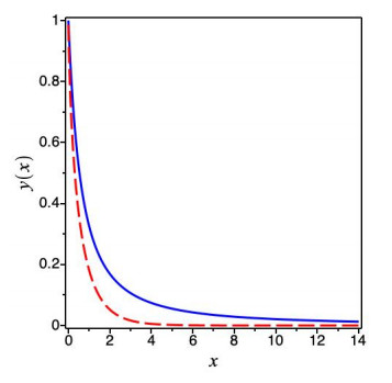
The existence and uniqueness theorem for the generalized boundary value problem of the Thomas-Fermi equation:

$ \begin{eqnarray*} \left\{ \begin{array}{l} y''+f(x, y) = 0, \ 0<x <\infty, \\ y(0) = 1, \ y(\infty) = 0, \end{array} \right. \end{eqnarray*} $

where

$ \begin{equation*} \label{6}f(x, y) = -y \left(\frac{y}{x}\right)^{\frac{p}{p+1}}, \ p>0, \ 0<x <\infty, \end{equation*} $

is proved. Also, highly accurate approximate solutions are obtained explicitly for this new boundary value problem which arises in particular studies of many-electron systems (atoms, ions, molecules, metals, crystals). To the best of our knowledge, the results obtained here are new and provide the lower and upper bounds approximate solutions for the generalized Thomas-Fermi problem.

References

[1]	L. H. Thomas, The calculation of atomic fields, Math. Proc. Cambridge Philos. Soc., 23 (1927), 542–548. https://doi.org/10.1017/S0305004100011683 doi: 10.1017/S0305004100011683
[2]	E. Fermi, Eine statistiche methode zur bestimmung einiger eigenschaften des atoms und ihre anwendung auf die theorie des periodischen systems der elemente, Z. Phys., 48 (1928), 73–79. https://doi.org/10.1007/BF01351576 doi: 10.1007/BF01351576
[3]	S. L. Shapiro, S. A. Teukolsky, Black holes, white dwarfs and neutron stars: the physics of compact objects, New York: Wiley, 1983. https://doi.org/10.1002/9783527617661
[4]	A. Sommerfeld, Integrazione asintotica dell'equazione differenziale di Thomas-Fermi, Rend. R. Accad. Lincei, 15 (1932), 293–308.
[5]	E. B. Baker, The application of the Fermi-Thomas statistical model to the calculation of potential distribution in positive ions, Phys. Rev., 36 (1930), 630–647. https://doi.org/10.1103/PhysRev.36.630 doi: 10.1103/PhysRev.36.630
[6]	V. Marinca, R. D. Ene, Analytical approximate solutions to the Thomas-Fermi equation, Cent. Eur. J. Phys., 12 (2014), 503–510. https://doi.org/10.2478/s11534-014-0472-9 doi: 10.2478/s11534-014-0472-9
[7]	A. A. Mavrin, A. V. Demura, Approximate solution of the Thomas-Fermi equation for free positive ions, Atoms, 9 (2021), 1–11. https://doi.org/10.3390/atoms9040087 doi: 10.3390/atoms9040087
[8]	A. Hasan-Zadeh, Examination of minimizer of Fermi energy in notions of Sobolev spaces, Res. J. Appl. Sci. Eng. Technol., 15 (2018), 356–361. http://dx.doi.org/10.19026/rjaset.15.5926 doi: 10.19026/rjaset.15.5926
[9]	H. Shababi, On the Thomas-Fermi model at the noncommutative framework, Eur. Phys. J. Plus, 137 (2022), 376. https://doi.org/10.1140/epjp/s13360-022-02596-9 doi: 10.1140/epjp/s13360-022-02596-9
[10]	H. Shababi, K. Ourabah, On the Thomas-Fermi model at the Planck scale, Phys. Lett. A, 383 (2019), 1105–1109. https://doi.org/10.1016/j.physleta.2019.01.019 doi: 10.1016/j.physleta.2019.01.019
[11]	H. Shababi, K. Ourabah, Thomas-Fermi theory at the Planck scale: a relativistic approach, Ann. Phys., 413 (2020), 168051. https://doi.org/10.1016/j.aop.2019.168051 doi: 10.1016/j.aop.2019.168051
[12]	M. Oulne, Variation and series approach to the Thomas-Fermi equation, Appl. Math. Comput., 218 (2011), 303–307. https://doi.org/10.1016/j.amc.2011.05.064 doi: 10.1016/j.amc.2011.05.064
[13]	J. P. Boyd, Rational Chebyshev series for the Thomas-Fermi function: endpoint singularities and spectral methods, J. Comput. Appl. Math., 244 (2013), 90–101. https://doi.org/10.1016/j.cam.2012.11.015 doi: 10.1016/j.cam.2012.11.015
[14]	K. Parand, A. Ghaderi, M. Delkhosh, H. Yousefi, A new approach for solving nonlinear Thomas-Fermi equation based on fractional order of rational Bessel functions, Electron. J. Differ. Equ., 331 (2016), 1–18. https://doi.org/10.48550/arXiv.1606.07615 doi: 10.48550/arXiv.1606.07615
[15]	K. Parand, K. Rabiei, M. Delkhosh, An efficient numerical method for solving nonlinear Thomas-Fermi equation, Acta Univ. Sapientiae Math., 10 (2018), 134–151. https://doi.org/10.2478/ausm-2018-0012 doi: 10.2478/ausm-2018-0012
[16]	S. V. Pikulin, Analytical-numerical method for calculating the Thomas-Fermi potential, Russ. J. Math. Phys., 26 (2019), 544–552. https://doi.org/10.1134/S1061920819040113 doi: 10.1134/S1061920819040113
[17]	L. Bougoffa, R. C. Rach, Approximate analytical solutions of the Thomas-Fermi equation by a direct method, Rom. Journ. Phys., 60 (2015), 1032–1039.
[18]	H. Fatoorehchi, H. Abolghasemi, An explicit analytic solution to the Thomas-Fermi Equation by the improved differential transform method, Acta Phys. Pol. A, 125 (2014), 1083–1087. https://doi.org/10.12693/APHYSPOLA.125.1083 doi: 10.12693/APHYSPOLA.125.1083
[19]	H. Fatoorehchi, M. Alidadi, The extended Laplace transform method for mathematical analysis of the Thomas-Fermi equation, Chin. J. Phys., 55 (2017), 2548–2558. https://doi.org/10.1016/j.cjph.2017.10.001 doi: 10.1016/j.cjph.2017.10.001
[20]	S. J. Liao, An explicit analytic solution to the Thomas-Fermi equation, Appl. Math. Comput., 144 (2003), 495–506. https://doi.org/10.1016/S0096-3003(02)00423-X doi: 10.1016/S0096-3003(02)00423-X
[21]	C. X. Liu, S. F. Zhu, Laguerre pseudospectral approximation to the Thomas-Fermi equation, J. Comput. Appl. Math., 282 (2015), 251–261. https://doi.org/10.1016/j.cam.2015.01.004 doi: 10.1016/j.cam.2015.01.004
[22]	S. F. Zhu, H. C. Zhu, Q. B. Wu, Y. Khan, An adaptive algorithm for the Thomas-Fermi equation, Numer. Algorithms, 59 (2012), 359-–372. https://doi.org/10.1007/s11075-011-9494-1 doi: 10.1007/s11075-011-9494-1
[23]	H. C. Rosu, S. C. Mancas, Generalized Thomas-Fermi equations as the Lampariello class of Emden-Fowler equations, Phys. A, 471 (2017), 212–218. https://doi.org/10.1016/j.physa.2016.12.007 doi: 10.1016/j.physa.2016.12.007
[24]	G. Adomian, Solving frontier problems of physics: the decomposition method, Dordrecht: Springer, 1994. https://doi.org/10.1007/978-94-015-8289-6
[25]	R. Rach, G. Adomian, Multiple decompositions for computational convenience, Appl. Math. Lett., 3 (1990), 97–99. https://doi.org/10.1016/0893-9659(90)90147-4 doi: 10.1016/0893-9659(90)90147-4
[26]	R. Rach, G. Adomian, R. E. Meyers, A modified decomposition, Comput. Math. Appl., 23 (1992), 17–23. https://doi.org/10.1016/0898-1221(92)90076-T doi: 10.1016/0898-1221(92)90076-T
[27]	G. Adomian, R. Rach, Transformations of series, Appl. Math. Lett., 4 (1991), 69–71. https://doi.org/10.1016/0893-9659(91)90058-4 doi: 10.1016/0893-9659(91)90058-4
[28]	J. S. Duan, R. Rach, A. M. Wazwaz, A new modified Adomian decomposition method for higher-order nonlinear dynamical systems, CMES, 94 (2013), 77–118. https://doi.org/10.3970/cmes.2013.094.077 doi: 10.3970/cmes.2013.094.077
[29]	L. Bougoffa, J. S. Duan, R. Rach, Exact and approximate analytic solutions of the thin film flow of fourth-grade fluids by the modified Adomian decomposition method, Int. J. Numer. Methods Heat Fluid Flow, 26 (2016), 2432–2440. https://doi.org/10.1108/HFF-07-2015-0278 doi: 10.1108/HFF-07-2015-0278
[30]	L. Bougoffa, S. Bougouffa, Adomian method for solving some coupled systems of two equations, Appl. Math. Comput., 177 (2006), 553–560. https://doi.org/10.1016/j.amc.2005.07.070 doi: 10.1016/j.amc.2005.07.070
[31]	L. Bougoffa, S. Bougouffa, Solutions of the two-wave interactions in quadratic nonlinear media, Mathematics, 8 (2020), 1–10. https://doi.org/10.3390/math8111867 doi: 10.3390/math8111867
[32]	L. Bougoffa, A. Mennouni, R. C. Rach, Solving Cauchy integral equations of the first kind by the Adomian decomposition method, Appl. Math. Comput., 219 (2013), 4423–4433. https://doi.org/10.1016/j.amc.2012.10.046 doi: 10.1016/j.amc.2012.10.046
[33]	A. M. Wazwaz, Partial differential equations and solitary waves theory, Berlin, Heidelberg: Springer, 2009. https://doi.org/10.1007/978-3-642-00251-9
[34]	M. van Hoeij, V. J. Kunwar, Classifying (almost)-Belyi maps with five exceptional points, Indagat. Math., 30 (2019), 136–156. https://doi.org/10.1016/j.indag.2018.09.003 doi: 10.1016/j.indag.2018.09.003
[35]	V. J. Kunwar, M. van Hoeij, Second order differential equations with hypergeometric solutions of degree three, In: Proceedings of the 38th International Symposium on Symbolic and Algebraic Computation, 2013,235–242. https://doi.org/10.1145/2465506.2465953
[36]	E. Imamoglu, M. van Hoeij, Computing hypergeometric solutions of second order linear differential equations using quotients of formal solutions and integral bases, J. Symb. Comput., 83 (2017), 254–271. https://doi.org/10.1016/j.jsc.2016.11.014 doi: 10.1016/j.jsc.2016.11.014
[37]	P. B. Bailey, L. F. Shampine, P. E. Waltman, Nonlinear two point boundary value problems, Academic Press, 1968.
[38]	W. M. Seiler, M. Seiss, On the numerical integration of singular initial and boundary value problems for generalized Lane-Emden and Thomas-Fermi equations, 2023, arXiv: 2301.01041v1.
[39]	C. Y. Chan, Y. C. Hon, Computational methods for generalized Thomas-Fermi models of neutral atoms, Q. Appl. Math., 46 (1988), 711–726.
[40]	J. Shahni, R. Singh, A fast numerical algorithm based on Chebyshev-wavelet technique for solving Thomas-Fermi type equation, Eng. Comput., 38 (2022), 3409–3422. https://doi.org/10.1007/s00366-021-01476-7 doi: 10.1007/s00366-021-01476-7
[41]	U. M. Ascher, R. M. M. Mattheij, R. D. Russell, Numerical solution of boundary value problems for ordinary differential equations, SIAM, 1995. https://doi.org/10.1137/1.9781611971231
[42]	U. M. Ascher, L. R. Petzold, Computer methods for ordinary differential equations and differential-algebraic equations, SIAM, 1998.

Reader Comments

Your name:*

Email:*
© 2023 the Author(s), licensee AIMS Press. This is an open access article distributed under the terms of the Creative Commons Attribution License (http://creativecommons.org/licenses/by/4.0)