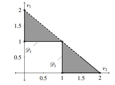
We consider the positivity of the discrete sequential fractional operators $ \left(^{\rm RL}_{a_{0}+1}\nabla^{\nu_{1}}\, ^{\rm RL}_{a_{0}}\nabla^{\nu_{2}}{f}\right)(\tau) $ defined on the set $ \mathscr{D}_{1} $ (see (1.1) and
Citation: Pshtiwan Othman Mohammed, Dumitru Baleanu, Thabet Abdeljawad, Soubhagya Kumar Sahoo, Khadijah M. Abualnaja. Positivity analysis for mixed order sequential fractional difference operators[J]. AIMS Mathematics, 2023, 8(2): 2673-2685. doi: 10.3934/math.2023140
We consider the positivity of the discrete sequential fractional operators $ \left(^{\rm RL}_{a_{0}+1}\nabla^{\nu_{1}}\, ^{\rm RL}_{a_{0}}\nabla^{\nu_{2}}{f}\right)(\tau) $ defined on the set $ \mathscr{D}_{1} $ (see (1.1) and

| [1] |
J. L. G. Guirao, P. O. Mohammed, H. M. Srivastava, D. Baleanu, M. S. Abualrub, Relationships between the discrete Riemann-Liouville and Liouville-Caputo fractional differences and their associated convexity results, AIMS Mathematics, 7 (2022), 18127–18141. https://doi.org/10.3934/math.2022997 doi: 10.3934/math.2022997

|
| [2] |
C. S. Goodrich, On discrete sequential fractional boundary value problems, J. Math. Anal. Appl., 385 (2012), 111–124. https://doi.org/10.1016/j.jmaa.2011.06.022 doi: 10.1016/j.jmaa.2011.06.022
|
| [3] |
T. Abdeljawad, Different type kernel $h$–fractional differences and their fractional $h$–sums, Chaos Soliton. Fract., 116 (2018), 146–156. https://doi.org/10.1016/j.chaos.2018.09.022 doi: 10.1016/j.chaos.2018.09.022
|
| [4] |
P. O. Mohammed, H. M. Srivastava, D. Baleanu, K. M. Abualnaja, Modified fractional difference operators defined using Mittag-Leffler kernels, Symmetry, 14 (2022), 1519. https://doi.org/10.3390/sym14081519 doi: 10.3390/sym14081519
|
| [5] |
F. M. Atici, M. Uyanik, Analysis of discrete fractional operators, Appl. Anal. Discr. Math., 9 (2015), 139–149. http://dx.doi.org/10.2298/AADM150218007A doi: 10.2298/AADM150218007A
|
| [6] |
F. M. Atici, M. Atici, M. Belcher, D. Marshall, A new approach for modeling with discrete fractional equations, Fund. Inform., 151 (2017), 313–324. http://dx.doi.org/10.3233/FI-2017-1494 doi: 10.3233/FI-2017-1494
|
| [7] |
F. M. Atici, S. S. Ayan, Modeling with fractional difference equations, J. Math. Anal. Appl., 369 (2010), 1–9. http://dx.doi.org/10.1016/j.jmaa.2010.02.009 doi: 10.1016/j.jmaa.2010.02.009
|
| [8] |
C. S. Goodrich, On discrete sequential fractional boundary value problems, J. Math. Anal. Appl., 385 (2012), 111–124. https://doi.org/10.1016/j.jmaa.2011.06.022 doi: 10.1016/j.jmaa.2011.06.022
|
| [9] |
C. R. Chen, M. Bohner, B. G. Jia, Ulam-hyers stability of Caputo fractional difference equations, Math. Methods Appl. Sci., 42 (2019), 7461–7470. https://doi.org/10.1002/mma.5869 doi: 10.1002/mma.5869
|
| [10] |
R. Dahal, C. S. Goodrich, Theoretical and numerical analysis of monotonicity results for fractional difference operators, Appl. Math. Lett., 117 (2021), 107104. https://doi.org/10.1016/j.aml.2021.107104 doi: 10.1016/j.aml.2021.107104
|
| [11] |
C. Lizama, The poisson distribution, abstract fractional difference equations, and stability, Proc. Amer. Math. Soc., 145 (2017), 3809–3827. http://dx.doi.org/10.1090/proc/12895 doi: 10.1090/proc/12895
|
| [12] |
H. M. Srivastava, P. O. Mohammed, C. S. Ryoo, Y. S. Hamed, Existence and uniqueness of a class of uncertain Liouville-Caputo fractional difference equations, J. King Saud Univ. Sci., 33 (2021), 101497. https://doi.org/10.1016/j.jksus.2021.101497 doi: 10.1016/j.jksus.2021.101497
|
| [13] |
Q. Lu, Y. Zhu, Comparison theorems and distributions of solutions to uncertain fractional difference equations, J. Cmput. Appl. Math., 376 (2020), 112884. https://doi.org/10.1016/j.cam.2020.112884 doi: 10.1016/j.cam.2020.112884
|
| [14] | F. M. Atici, P. W. Eloe, A transform method in discrete fractional calculus, Int. J. Differ. Equ., 2 (2007), 165–176. |
| [15] | P. O. Mohammed, T. Abdeljawad, Discrete generalized fractional operators defined using $h$-discrete Mittag-Leffler kernels and applications to AB fractional difference systems, Math. Methods Appl. Sci., 2020. https://doi.org/10.1002/mma.7083 |
| [16] | F. M. Atici, M. Atici, N. Nguyen, T. Zhoroev, G. Koch, A study on discrete and discrete fractional pharmaco kinetics pharmaco dynamics models for tumor growth and anti-cancer effects, Comput. Math. Biophys., 7 (2019), 10–24. |
| [17] |
A. Silem, H. Wu, D. J. Zhang, Discrete rogue waves and blow-up from solitons of a nonisospectral semi-discrete nonlinear Schrödinger equation, Appl. Math. Lett., 116 (2021), 107049. https://doi.org/10.1016/j.aml.2021.107049 doi: 10.1016/j.aml.2021.107049
|
| [18] |
R. A. C. Ferreira, D. F. M. Torres, Fractional h-difference equations arising from the calculus of variations, Appl. Anal. Discrete Math., 5 (2011), 110–121. https://doi.org/10.2298/AADM110131002F doi: 10.2298/AADM110131002F
|
| [19] |
G. C. Wu, D. Baleanu, Discrete chaos in fractional delayed logistic maps, Nonlinear Dyn., 80 (2015), 1697–1703. http://dx.doi.org/10.1007/s11071-014-1250-3 doi: 10.1007/s11071-014-1250-3
|
| [20] |
J. W. He, L. Zhang, Y. Zhou, B. Ahmad, Existence of solutions for fractional difference equations via topological degree methods, Adv. Differ. Equ., 2018 (2018), 153. https://doi.org/10.1186/s13662-018-1610-2 doi: 10.1186/s13662-018-1610-2
|
| [21] |
R. Dahal, C. S. Goodrich, A monotonicity result for discrete fractional difference operators, Arch. Math. (Basel), 102 (2014), 293–299. https://doi.org/10.1007/S00013-014-0620-X doi: 10.1007/S00013-014-0620-X
|
| [22] |
C. S. Goodrich, B. Lyons, Positivity and monotonicity results for triple sequential fractional differences via convolution, Analysis, 40 (2020), 89–103. http://dx.doi.org/10.1515/anly-2019-0050 doi: 10.1515/anly-2019-0050
|
| [23] |
P. O. Mohammed, T. Abdeljawad, F. K. Hamasalh, On Riemann-Liouville and Caputo fractional forward difference monotonicity analysis, Mathematics, 9 (2021), 1303. https://doi.org/10.3390/math9111303 doi: 10.3390/math9111303
|
| [24] |
P. O. Mohammed, T. Abdeljawad, F. K. Hamasalh, On Discrete delta Caputo-Fabrizio fractional operators and monotonicity analysis, Fractal Fract., 5 (2021), 116. https://doi.org/10.3390/fractalfract5030116 doi: 10.3390/fractalfract5030116
|
| [25] |
T. Abdeljawad, D. Baleanu, Monotonicity analysis of a nabla discrete fractional operator with discrete Mittag-Leffler kernel, Chaos Soliton. Fract., 102 (2017), 106–110. https://doi.org/10.1016/j.chaos.2017.04.006 doi: 10.1016/j.chaos.2017.04.006
|
| [26] |
X. Liu, F. F. Du, D. R. Anderson, B. Jia, Monotonicity results for nabla fractional h-difference operators, Math. Methods Appl. Sci., 44 (2020), 1207–1218. https://doi.org/10.1002/mma.6823 doi: 10.1002/mma.6823
|
| [27] |
R. Dahal, C. S. Goodrich, B. Lyons, Monotonicity results for sequential fractional differences of mixed orders with negative lower bound, J. Differ. Equ. Appl., 27 (2021), 1574–1593. https://doi.org/10.1080/10236198.2021.1999434 doi: 10.1080/10236198.2021.1999434
|
| [28] |
P. O. Mohammed, O. Almutairi, R. P. Agarwal, Y. S. Hamed, On convexity, monotonicity and positivity analysis for discrete fractional operators defined using exponential kernels, Fractal Fract., 6 (2022), 55. https://doi.org/10.3390/fractalfract6020055 doi: 10.3390/fractalfract6020055
|
| [29] |
C. S. Goodrich, J. M. Jonnalagadda, Monotonicity results for CFC nabla fractional differences with negative lower bound, Analysis, 44 (2021), 221–229. https://doi.org/10.1515/anly-2021-0011 doi: 10.1515/anly-2021-0011
|
| [30] | C. S. Goodrich, Monotonicity and non-monotonicity results for sequential fractional delta differences of mixed order, Analysis, 22 (2018). https://doi.org/10.1007/S11117-017-0527-4 |
| [31] |
P. O. Mohammed, C. S. Goodrich, F. K. Hamasalh, A. Kashuri, Y. S. Hamed, On positivity and monotonicity analysis for discrete fractional operators with discrete Mittag-Leffler kernel, Math. Methods Appl. Sci., 45 (2022), 6931–6410. https://doi.org/10.1002/mma.8176 doi: 10.1002/mma.8176
|
| [32] | C. S. Goodrich, A. C. Peterson, Discrete fractional calculus, Springer, 2015. |

Figures(2)

Pshtiwan Othman Mohammed, Dumitru Baleanu, Thabet Abdeljawad, Soubhagya Kumar Sahoo, Khadijah M. Abualnaja. Positivity analysis for mixed order sequential fractional difference operators[J]. AIMS Mathematics, 2023, 8(2): 2673-2685. doi: 10.3934/math.2023140


 DownLoad: