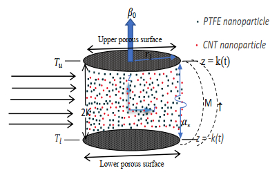
The objective of this study is to explore the heat transfer properties and flow features of an MHD hybrid nanofluid due to the dispersion of polymer/CNT matrix nanocomposite material through orthogonal permeable disks with the impact of morphological nanolayer. Matrix nanocomposites (MNC) are high-performance materials with unique properties and design opportunities. These MNC materials are beneficial in a variety of applications, spanning from packaging to biomedical applications, due to their exceptional thermophysical properties. The present innovative study is the dispersion of polymeric/ceramic matrix nanocomposite material on magnetized hybrid nanofluids flow through the orthogonal porous coaxial disks is deliberated. Further, we also examined the numerically prominence of the permeability ($ {\mathrm{A}}_{\mathrm{*}} $) function consisting of the Permeable Reynold number associated with the expansion/contraction ratio. The morphological significant effects of these nanomaterials on flow and heat transfer characteristics are explored. The mathematical structure, as well as empirical relations for nanocomposite materials, are formulated as partial differential equations, which are then translated into ordinary differential expressions using appropriate variables. The Runge–Kutta and shooting methods are utilized to find the accurate numerical solution. Variations in skin friction coefficient and Nusselt number at the lower and upper walls of disks, as well as heat transfer rate measurements, are computed using important engineering physical factors. A comparison table and graph of effective nanolayer thermal conductivity (ENTC) and non-effective nanolayer thermal conductivity are presented. It is observed that the increment in nanolayer thickness (0.4−1.6), enhanced the ENTC and thermal phenomena. By the enhancement in hybrid nanoparticles volume fraction (2% to 6%), significant enhancement in Nusselt number is noticed. This novel work may be beneficial for nanotechnology and relevant nanocomponents.
Citation: M Zubair Akbar Qureshi, M Faisal, Qadeer Raza, Bagh Ali, Thongchai Botmart, Nehad Ali Shah. Morphological nanolayer impact on hybrid nanofluids flow due to dispersion of polymer/CNT matrix nanocomposite material[J]. AIMS Mathematics, 2023, 8(1): 633-656. doi: 10.3934/math.2023030
The objective of this study is to explore the heat transfer properties and flow features of an MHD hybrid nanofluid due to the dispersion of polymer/CNT matrix nanocomposite material through orthogonal permeable disks with the impact of morphological nanolayer. Matrix nanocomposites (MNC) are high-performance materials with unique properties and design opportunities. These MNC materials are beneficial in a variety of applications, spanning from packaging to biomedical applications, due to their exceptional thermophysical properties. The present innovative study is the dispersion of polymeric/ceramic matrix nanocomposite material on magnetized hybrid nanofluids flow through the orthogonal porous coaxial disks is deliberated. Further, we also examined the numerically prominence of the permeability ($ {\mathrm{A}}_{\mathrm{*}} $) function consisting of the Permeable Reynold number associated with the expansion/contraction ratio. The morphological significant effects of these nanomaterials on flow and heat transfer characteristics are explored. The mathematical structure, as well as empirical relations for nanocomposite materials, are formulated as partial differential equations, which are then translated into ordinary differential expressions using appropriate variables. The Runge–Kutta and shooting methods are utilized to find the accurate numerical solution. Variations in skin friction coefficient and Nusselt number at the lower and upper walls of disks, as well as heat transfer rate measurements, are computed using important engineering physical factors. A comparison table and graph of effective nanolayer thermal conductivity (ENTC) and non-effective nanolayer thermal conductivity are presented. It is observed that the increment in nanolayer thickness (0.4−1.6), enhanced the ENTC and thermal phenomena. By the enhancement in hybrid nanoparticles volume fraction (2% to 6%), significant enhancement in Nusselt number is noticed. This novel work may be beneficial for nanotechnology and relevant nanocomponents.

| [1] |
L. F. Tóth, P. De. Baets, G. Szebényi, Thermal, viscoelastic, mechanical and wear behaviour of nanoparticle filled polytetrafluoroethylene: A comparison, Polymers, 12 (2020), 1940. https://doi.org/10.3390/polym12091940 doi: 10.3390/polym12091940

|
| [2] |
W. E. Hanford, R. M. Joyce, Polytetrafluoroethylene, J. Am. Chem. Soc., 68 (1946), 2082−2085. https://doi.org/10.1021/ja01214a062 doi: 10.1021/ja01214a062
|
| [3] | V. Choudhary, A. Gupta, Polymer/carbon nanotube nanocomposites, In: Carbon nanotubes-polymer nanocomposites, London: IntechOpen, 2011. https://doi.org/10.5772/18423 |
| [4] |
W. X. Chen, F. Li, G. Han, J. B. Xia, L. Y. Wang, J. P. Tu, et al., Tribological behavior of carbon-nanotube-filled PTFE composites, Tribol. Lett., 15 (2003), 275−278. https://doi.org/10.1023/A:1024869305259 doi: 10.1023/A:1024869305259
|
| [5] |
Y. Lin, B. Zhou, K. A. Shiral Fernando, P. Liu, L. F. Allard, Y. P. Sun, Polymeric carbon nanocomposites from carbon nanotubes functionalized with matrix polymer, Macromolecules, 36 (2003), 7199−7204. https://doi.org/10.1021/ma0348876 doi: 10.1021/ma0348876
|
| [6] |
C. J. Yu, A. G. Richter, A. Datta, M. K. Durbin, P. Dutta, Molecular layering in a liquid on a solid substrate: an X-ray reflectivity study, Physica B., 283 (2000), 27−31. https://doi.org/10.1016/S0921-4526(99)01885-2 doi: 10.1016/S0921-4526(99)01885-2
|
| [7] |
W. Yu, S. U. S. Choi, The role of interfacial layers in the enhanced thermal conductivity of nanofluids: a renovated Hamilton–Crosser model, J. Nanopart. Res., 6 (2004), 355−361. https://doi.org/10.1007/s11051-004-2601-7 doi: 10.1007/s11051-004-2601-7
|
| [8] |
Q. Z. Xue, Model for effective thermal conductivity of nanofluids, Phys. Lett. A, 307 (2003), 313−317. https://doi.org/10.1016/S0375-9601(02)01728-0 doi: 10.1016/S0375-9601(02)01728-0
|
| [9] |
W. Yu, S. U. S. Choi, The role of interfacial layers in the enhanced thermal conductivity of nanofluids: a renovated Maxwell model, J. Nanopart. Res., 5 (2003), 167−171. https://doi.org/10.1023/A:1024438603801 doi: 10.1023/A:1024438603801
|
| [10] |
M. Z. A. Qureshi, S. Bilal, M. Y. Malik, Q. Raza, E. S. M. Sherif, Y. M. Li, Dispersion of metallic/ceramic matrix nanocomposite material through porous surfaces in magnetized hybrid nanofluids flow with shape and size effects, Sci. Rep., 11 (2021), 12271. https://doi.org/10.1038/s41598-021-91152-z doi: 10.1038/s41598-021-91152-z
|
| [11] |
Z. Abdelmalek, M. Z. A. Qureshi, S. Bilal, Q. Raza, E. S. M. Sherif, A case study on morphological aspects of distinct magnetized 3D hybrid nanoparticles on fluid flow between two orthogonal rotating disks: An application of thermal energy systems, Case Stud. Therm. Eng., 23 (2021), 100744. https://doi.org/10.1016/j.csite.2020.100744 doi: 10.1016/j.csite.2020.100744
|
| [12] |
N. Bachok, A. Ishak, I. Pop, Flow and heat transfer over a rotating porous disk in a nanofluid, Physica B, 406 (2011), 1767−1772. https://doi.org/10.1016/j.physb.2011.02.024 doi: 10.1016/j.physb.2011.02.024
|
| [13] |
M. Z. A. Qureshi, K. Ali, M. F. Iqbal, M. Ashraf, Heat and mass transfer analysis of unsteady non-newtonian fluid flow between porous surfaces in the presence of magnetic nanoparticles, J. Porous Media, 20 (2017), 1137−1154. https://doi.org/10.1615/JPorMedia.v20.i12.60 doi: 10.1615/JPorMedia.v20.i12.60
|
| [14] |
S. Bilal, M. Z. A. Qureshi, Mathematical analysis of hybridized ferromagnetic nanofluid with induction of copper oxide nanoparticles in permeable channel by incorporating Darcy–Forchheimer relation, Math. Sci., 2021. https://doi.org/10.1007/s40096-021-00421-5 doi: 10.1007/s40096-021-00421-5
|
| [15] |
H. Alfven, Existance of electromagnetic-hydrodynamic waves, Nature, 150 (1942), 405−406. https://doi.org/10.1038/150405d0 doi: 10.1038/150405d0
|
| [16] |
E. H. Aly, I. Pop, MHD flow and heat transfer over a permeable stretching/shrinking sheet in a hybrid nanofluid with a convective boundary condition, Int. J. Numer. Method. H., 29 (2019), 3012−3038. https://doi.org/10.1108/HFF-12-2018-0794 doi: 10.1108/HFF-12-2018-0794
|
| [17] |
A. J. Chamkha, A. S. Dogonchi, D. D. Ganji, Magnetohydrodynamic nanofluid natural convection in a cavity under thermal radiation and shape factor of nanoparticles impacts: a numerical study using CVFEM, Appl. Sci., 8 (2018), 2396. https://doi.org/10.3390/app8122396 doi: 10.3390/app8122396
|
| [18] |
A. S. Dogonchi, D. D. Ganji, Investigation of heat transfer for cooling turbine disks with a non-Newtonian fluid flow using DRA, Case Stud. Therm. Eng., 6 (2015), 40−51. https://doi.org/10.1016/j.csite.2015.06.002 doi: 10.1016/j.csite.2015.06.002
|
| [19] |
M. V. Krishna, Heat transport on steady MHD flow of copper and alumina nanofluids past a stretching porous surface, Heat Transf., 49 (2020), 1374-1385. https://doi.org/10.1002/htj.21667 doi: 10.1002/htj.21667
|
| [20] |
S. P. A. Devi, S. S. U. Devi, Numerical investigation of hydromagnetic hybrid Cu–Al2O3/water nanofluid flow over a permeable stretching sheet with suction, Int. J. Nonlin. Sci. Num., 17 (2016), 249−257. https://doi.org/10.1515/ijnsns-2016-0037 doi: 10.1515/ijnsns-2016-0037
|
| [21] |
M. V. Krishna, N. A. Ahammad, A. J. Chamkha, Radiative MHD flow of Casson hybrid nanofluid over an infinite exponentially accelerated vertical porous surface, Case Stud. Therm. Eng., 27 (2021), 101229. https://doi.org/10.1016/j.csite.2021.101229 doi: 10.1016/j.csite.2021.101229
|
| [22] |
N. Abbas, K. U. Rehman, W. Shatanawi, M. Y. Malik, Numerical study of heat transfer in hybrid nanofluid flow over permeable nonlinear stretching curved surface with thermal slip, Int. Commun. Heat. Mass., 135 (2022), 106107. https://doi.org/10.1016/j.icheatmasstransfer.2022.106107 doi: 10.1016/j.icheatmasstransfer.2022.106107
|
| [23] |
H. Upreti, A. K. Pandey, M. Kumar, Unsteady squeezing flow of magnetic hybrid nanofluids within parallel plates and entropy generation, Heat Transf., 50 (2021), 105−125. https://doi.org/10.1002/htj.21994 doi: 10.1002/htj.21994
|
| [24] |
H. Upreti, A. K. Pandey, M. Kumar, Assessment of entropy generation and heat transfer in three-dimensional hybrid nanofluids flow due to convective surface and base fluids, J. Porous Media, 24 (2021), 35−50. https://doi.org/10.1615/JPorMedia.2021036038 doi: 10.1615/JPorMedia.2021036038
|
| [25] |
N. Abbas, S. Nadeem, A. Saleem, Computational analysis of water based Cu-Al2O3/H2O flow over a vertical wedge, Adv. Mech. Eng., 12 (2020). https://doi.org/10.1177/1687814020968322 doi: 10.1177/1687814020968322
|
| [26] |
S. Nadeem, A. Amin, N. Abbas, On the stagnation point flow of nanomaterial with base viscoelastic micropolar fluid over a stretching surface, Alex. Eng. J., 59 (2020), 1751−1760. https://doi.org/10.1016/j.aej.2020.04.041 doi: 10.1016/j.aej.2020.04.041
|
| [27] |
M. I. Anwar, H. Firdous, A. A. Zubaidi, N. Abbas, S. Nadeem, Computational analysis of induced magnetohydrodynamic non-Newtonian nanofluid flow over nonlinear stretching sheet, Prog. React. Kinet. Mec., 47 (2022). https://doi.org/10.1177/14686783211072712 doi: 10.1177/14686783211072712
|
| [28] |
P. Priyadharshini, M. V. Archana, N. A. Ahammad, C. S. K. Raju, S. J. Yook, N. A. Shah, Gradient descent machine learning regression for MHD flow: Metallurgy process, Int. Commun. Heat. Mass., 138 (2022), 106307. https://doi.org/10.1016/j.icheatmasstransfer.2022.106307 doi: 10.1016/j.icheatmasstransfer.2022.106307
|
| [29] |
N. A. Shah, A. Wakif, E. R. El-Zahar, S. Ahmad, S. J. Yook, Numerical simulation of a thermally enhanced EMHD flow of a heterogeneous micropolar mixture comprising (60%)-ethylene glycol (EG), (40%)-water (W), and copper oxide nanomaterials (CuO), Case Stud. Therm. Eng., 35 (2022), 102046. https://doi.org/10.1016/j.csite.2022.102046 doi: 10.1016/j.csite.2022.102046
|
| [30] |
K. Sajjan, N. A. Shah, N. A. Ahammad, C. S. K. Raju, M. D. Kumar, W. Weera, Nonlinear Boussinesq and Rosseland approximations on 3D flow in an interruption of Ternary nanoparticles with various shapes of densities and conductivity properties, AIMS Mathematics, 7 (2022), 18416−18449. https://doi.org/10.3934/math.20221014 doi: 10.3934/math.20221014
|
| [31] |
Q. Raza, M. Z. A. Qureshi, B. A. Khan, A. K. Hussein, B. Ali, N. A. Shah, et al., Insight into dynamic of mono and hybrid nanofluids subject to binary chemical reaction, activation energy, and magnetic field through the porous surfaces, Mathematics, 10 (2022), 3013. https://doi.org/10.3390/math10163013 doi: 10.3390/math10163013
|
| [32] |
A.S. Sabu, A. Wakif, S. Areekara, A. Mathew, N.A. Shah, Significance of nanoparticles' shape and thermo-hydrodynamic slip constraints on MHD alumina-water nanoliquid flows over a rotating heated disk: the passive control approach, Int. Commun. Heat Mass Transf., 129 (2021) 105711. https://doi.org/10.1016/j.icheatmasstransfer.2021.105711 doi: 10.1016/j.icheatmasstransfer.2021.105711
|
| [33] |
T. C. Zhang, Q. L. Zou, Z. H. Cheng, Z. H. Chen, Y. Liu, Z. B. Jiang, Effect of particle concentration on the stability of water-based SiO2 nanofluid, Powder Technol., 379 (2021), 457−465. https://doi.org/10.1016/j.powtec.2020.10.073 doi: 10.1016/j.powtec.2020.10.073
|
| [34] |
T. Oreyeni, N. A. Shah, A. O. Popoola, E. R. Elzahar, S. J. Yook, The significance of exponential space-based heat generation and variable thermophysical properties on the dynamics of Casson fluid over a stratified surface with nonuniform thickness, Wave. Random. Complex., 2022, 1−19. https://doi.org/10.1080/17455030.2022.2119304 doi: 10.1080/17455030.2022.2119304
|
| [35] |
K. Ali, M. F. Iqbal, Z. Akbar, M. Ashraf, Numerical simulation of unsteady water-based nanofluid flow and heat transfer between two orthogonally moving porous coaxial disks, J. Theor. App. Mech., 52 (2014), 1033−1046. https://doi.org/10.15632/jtam-pl.52.4.1033 doi: 10.15632/jtam-pl.52.4.1033
|
| [36] |
J. Majdalani, C. Zhou, C. A. Dawson, Two-dimensional viscous flow between slowly expanding or contracting walls with weak permeability, J. Biomech., 35 (2002) 1399–1403. https://doi.org/10.1016/S0021-9290(02)00186-0 doi: 10.1016/S0021-9290(02)00186-0
|
| [37] |
Q. Lou, B. Ali, S. U. Rehman, D. Habib, S. Abdal, N. A. Shah, et al., Micropolar dusty fluid: coriolis force effects on dynamics of MHD rotating fluid when lorentz force is significant, Mathematics, 10 (2022), 2630. https://doi.org/10.3390/math10152630 doi: 10.3390/math10152630
|
| [38] |
M. Z. Ashraf, S. U. Rehman, S. Farid, A. K. Hussein, B. Ali, N. A. Shah, et al., Insight into significance of bioconvection on MHD tangent hyperbolic nanofluid flow of irregular thickness across a slender elastic surface, Mathematics, 10 (2022), 2592. https://doi.org/10.3390/math10152592 doi: 10.3390/math10152592
|
| [39] |
M. Gupta, V. Singh, R. Kumar, Z. Said, A review on thermophysical properties of nanofluids and heat transfer applications, Renew. Sust. Energ. Rev., 74 (2017), 638−670. https://doi.org/10.1016/j.rser.2017.02.073 doi: 10.1016/j.rser.2017.02.073
|
| [40] |
L. Yang, W. K. Ji, J. N. Huang, G. Y. Xu, An updated review on the influential parameters on thermal conductivity of nano-fluids, J. Mol. Liq., 296 (2019), 111780. https://doi.org/10.1016/j.molliq.2019.111780 doi: 10.1016/j.molliq.2019.111780
|
| [41] |
M. L. Levin, M. A. Miller, Maxwell's "treatise on electricity and magnetism", Sov. Phys. Usp., 24 (1981), 904. https://doi.org/10.1070/PU1981V024N11ABEH004793 doi: 10.1070/PU1981V024N11ABEH004793
|
| [42] |
R. L. Hamilton, O. K. Crosser, Thermal conductivity of heterogeneous two-component systems, Ind. Eng. Chem. Fundament., 1 (1962), 187−191. https://doi.org/10.1021/i160003a005 doi: 10.1021/i160003a005
|
| [43] |
H. F. Jiang, Q. H. Xu, C. Huang, L. Shi, The role of interfacial nanolayer in the enhanced thermal conductivity of carbon nanotube-based nanofluids, Appl. Phys. A, 118 (2015), 197−205. https://doi.org/10.1007/s00339-014-8902-5 doi: 10.1007/s00339-014-8902-5
|
| [44] |
S. M. S. Murshed, K. C. Leong, C. Yang, Investigations of thermal conductivity and viscosity of nanofluids, Int. J. Therm. Sci., 47 (2008), 560−568. https://doi.org/10.1016/j.ijthermalsci.2007.05.004 doi: 10.1016/j.ijthermalsci.2007.05.004
|


Figures(10) / Tables(9)

M Zubair Akbar Qureshi, M Faisal, Qadeer Raza, Bagh Ali, Thongchai Botmart, Nehad Ali Shah. Morphological nanolayer impact on hybrid nanofluids flow due to dispersion of polymer/CNT matrix nanocomposite material[J]. AIMS Mathematics, 2023, 8(1): 633-656. doi: 10.3934/math.2023030


 DownLoad: