Galerkin time discretization scheme for the transmission dynamics of HIV infection with non-linear supply rate

Attaullah; Ramzi Drissi; Wajaree Weera; Attaullah; Ramzi Drissi; Wajaree Weera

doi:10.3934/math.2022630

AIMS Mathematics

2022, Volume 7, Issue 6: 11292-11310. doi: 10.3934/math.2022630

Previous Article Next Article

Research article Special Issues

Galerkin time discretization scheme for the transmission dynamics of HIV infection with non-linear supply rate

1.
Department of Mathematics and Statistics, Bacha Khan University, Charsadda 24420, Pakistan
2.
Department of Insurance, College of Islamic Economics and Finance, Umm Al-Qura University, Makkah, 24243, Saudi Arabia
3.
Department of Mathematics, Faculty of Science, Khon Kaen University, Khon Kaen, 40002, Thailand

Received: 17 December 2021 Revised: 19 March 2022 Accepted: 28 March 2022 Published: 11 April 2022
MSC : 34A12, 34K28

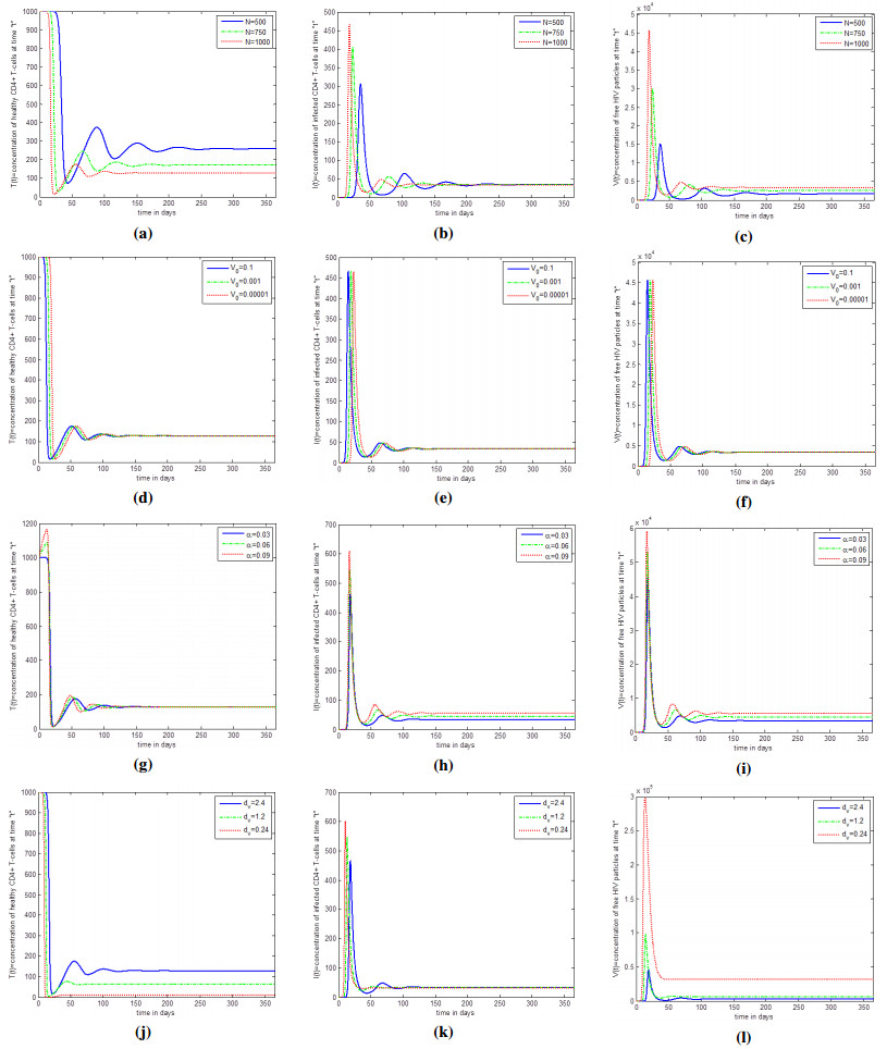
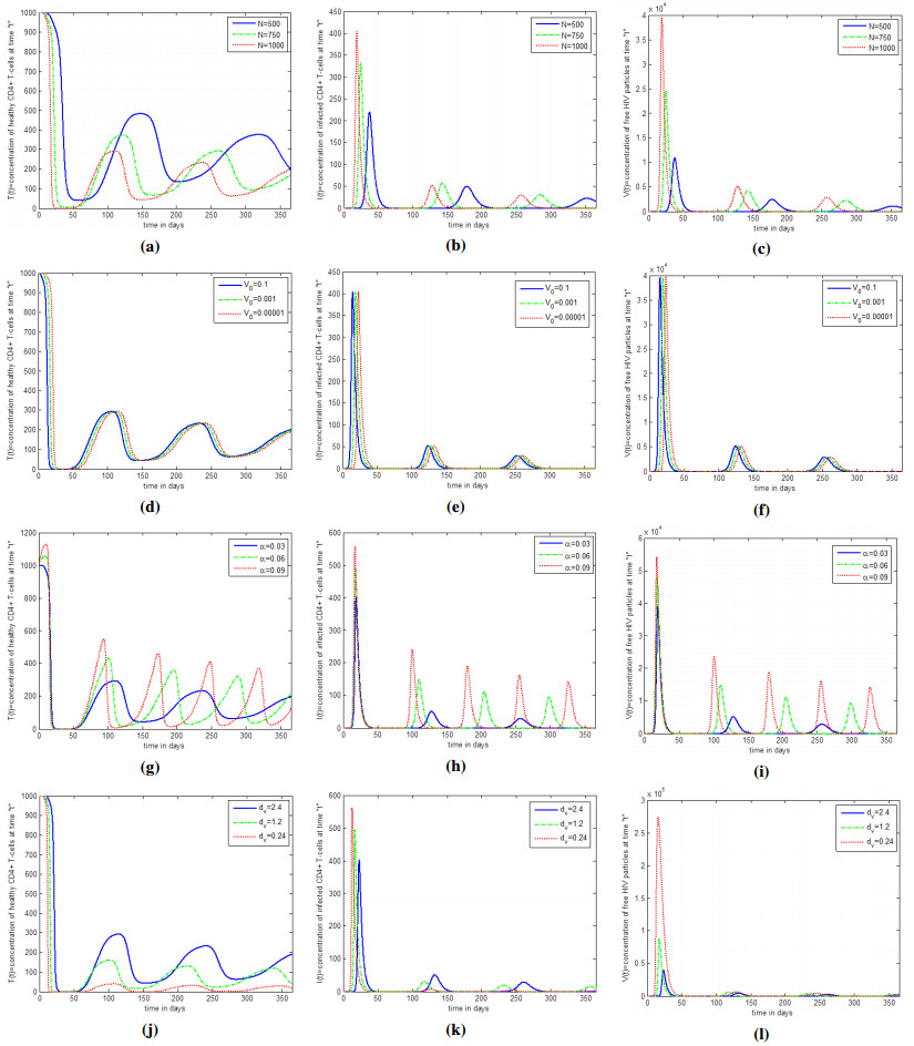
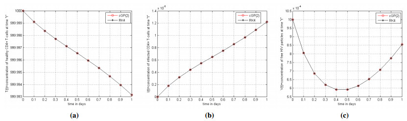
The present work implements the continuous Galerkin-Petrov method (cGP(2)-method) to compute an approximate solution of the model for HIV infection of $ \text{CD4}^{+} $ T-cells. We discuss and analyse the influence of different clinical parameters on the model. The work also depicts graphically that how the level of $ \text{CD4}^{+} $ T-cells varies with respect to the emerging parameters in the model. Simultaneously, the model is solved using the fourth-order Runge Kutta (RK4) method. Finally, the validity and reliability of the proposed scheme are verified by comparing the numerical and graphical results with those obtained through the RK4 method. A numerical comparison between the results of the cGP (2) method and the RK4 method reveals that the proposed technique is a promising tool for the approximate solution of non-linear systems of differential equations. The present study highlights the accuracy and efficiency of the proposed schemes as in comparison to the other traditional schemes, for example, the Laplace adomian decomposition method (LADM), variational iteration method (VIM), homotopy analysis method (HAM), homotopy perturbation method (HAPM), etc. In this study, two different versions of the HIV model are considered. In the first one, the supply of new $ \text{CD4}^{+} $ T-cells from the thymus is constant, while in the second, we consider the production of these cells as a monotonically decreasing function of viral load. The experiments show that the lateral model provides more reasonable predictions than the former model.
- HIV infection,
- CD4$ ^{+} $ T-cells,
- continuous Galerkin-Petrov method,
- non-linear supply rate
Citation: Attaullah, Ramzi Drissi, Wajaree Weera. Galerkin time discretization scheme for the transmission dynamics of HIV infection with non-linear supply rate[J]. AIMS Mathematics, 2022, 7(6): 11292-11310. doi: 10.3934/math.2022630

Related Papers:

Abstract

The present work implements the continuous Galerkin-Petrov method (cGP(2)-method) to compute an approximate solution of the model for HIV infection of $ \text{CD4}^{+} $ T-cells. We discuss and analyse the influence of different clinical parameters on the model. The work also depicts graphically that how the level of $ \text{CD4}^{+} $ T-cells varies with respect to the emerging parameters in the model. Simultaneously, the model is solved using the fourth-order Runge Kutta (RK4) method. Finally, the validity and reliability of the proposed scheme are verified by comparing the numerical and graphical results with those obtained through the RK4 method. A numerical comparison between the results of the cGP (2) method and the RK4 method reveals that the proposed technique is a promising tool for the approximate solution of non-linear systems of differential equations. The present study highlights the accuracy and efficiency of the proposed schemes as in comparison to the other traditional schemes, for example, the Laplace adomian decomposition method (LADM), variational iteration method (VIM), homotopy analysis method (HAM), homotopy perturbation method (HAPM), etc. In this study, two different versions of the HIV model are considered. In the first one, the supply of new $ \text{CD4}^{+} $ T-cells from the thymus is constant, while in the second, we consider the production of these cells as a monotonically decreasing function of viral load. The experiments show that the lateral model provides more reasonable predictions than the former model.

References

[1]	S. Perelson, Modeling the interaction of the immune system with HIV, In: Mathematical and statistical approaches to AIDS epidemiology, Berlin: Springer, 1989,350–370. https://doi.org/10.1007/978-3-642-93454-4_17
[2]	A. S. Perelson, D. E. Kirschner, R. De Boer, Dynamics of HIV infection of CD$4^{+}$ T-cells, Math. Biosci., 114 (1993), 81–125. https://doi.org/10.1016/0025-5564(93)90043-a doi: 10.1016/0025-5564(93)90043-a
[3]	R. V. Culshaw, S. Ruan, A delay- differential equation model of HIV infection of CD$4^{+}$ T-cells, Math. Biosci., 165 (2000), 27–39. https://doi.org/10.1016/S0025-5564(00)00006-7 doi: 10.1016/S0025-5564(00)00006-7
[4]	X. Wang, X. Song, Global stability and periodic solution of a model for HIV infection of CD$4^{+}$ T-cells, Appl. Math. Comput., 189 (2007), 1331–1340. https://doi.org/10.1016/j.amc.2006.12.044 doi: 10.1016/j.amc.2006.12.044
[5]	M. S. Mechee, N. Haitham, Application of lie symmetry for mathematical model of HIV infection of CD$4^+$ t-cells, Int. J. Appl. Eng. Res., 13 (2018), 5069–5074.
[6]	Q. Li, Y. Xiao, Global dynamics of a virus immune system with virus guided therapy and saturation growth of virus, J. Mathe. Prob. Engi., 2018 (2018), 4710586. https://doi.org/10.1155/2018/4710586 doi: 10.1155/2018/4710586
[7]	L. J. G. Lima, M. S. Espindola, L. S. Soares, F. A. Zambuzi, M. Cacemiro, C. Fontanari, et al. Classical and alternative macrophages have impaired function during acute and chronic HIV-1 infection, Braz. J. Infect. Dis., 21 (2017), 42–50. https://doi.org/10.1016/j.bjid.2016.10.004 doi: 10.1016/j.bjid.2016.10.004
[8]	S. A. Kinner, K. Snow, A. L. Wirtz, F. L. Altice, C. Beyrer, K. Dolan, et al. Age-specific global prevalence of hepatitis B, hepatitis C, HIV and tuberculosis among incarcerated people: A systematic review, J. Math. Biol., 62 (2018), 18–26. https://doi.org/10.1016/j.jadohealth.2017.09.030 doi: 10.1016/j.jadohealth.2017.09.030
[9]	J. M. C. Angulo, T. A. C. Cuesta, E. P. Menezes, C. Pedroso, C. Brites, A systematic review on the influence of HLA-B polymorphisms on HIV-1 mother to child transmission, Braz. J. Infect. Dis., 23 (2019), 53–59. https://doi.org/10.1016/j.bjid.2018.12.002 doi: 10.1016/j.bjid.2018.12.002
[10]	K. Theys, P. Libin, A. C. P. Pena, A. Nowe, A. M. Vandamme, A. B. Abecasis, The impact of HIV-1 within host evolution on transmission dynamics, Curr. Opin. Virol., 28 (2018), 92–101. https://doi.org/10.1016/j.coviro.2017.12.001 doi: 10.1016/j.coviro.2017.12.001
[11]	D. Hallberg, T. D. Kimario, C. Mtuya, M. Msuya, G. Bjorling, Factors affecting HIV disclosure among partners in morongo, tanzania, Int. J. Afr. Nurs. Sci., 10 (2019), 49–54. https://doi.org/10.1016/j.ijans.2019.01.006 doi: 10.1016/j.ijans.2019.01.006
[12]	Y. Ransome, K. A. Thurber, M. Swen, N. D. Crawford, D. Germane, L. T. Dean, Social capital and HIV/AIDS in the united states: Knowledge, gaps and future directions, SSM-Popul. Heal., 5 (2018), 73–85. https://doi.org/10.1016/j.ssmph.2018.05.007 doi: 10.1016/j.ssmph.2018.05.007
[13]	K. Naidoo, S. Gengiah, S. Singh, J. Stillo, N. Padayatchi, Quality of tb care among people living with HIV: Gaps and solutions, J. liCnical Tuberc. Mycobacterial Dis., 17 (2019), 100122. https://doi.org/10.1016/j.jctube.2019.100122 doi: 10.1016/j.jctube.2019.100122
[14]	E. O. Omondi, W. R. Mbogo, L. S. Luboobi, A mathematical modeling study of HIV infection in two heterosexual age groups in kenya, J. Infect. Dis. Model., 4 (2019), 83–98. https://doi.org/10.1016/j.idm.2019.04.003 doi: 10.1016/j.idm.2019.04.003
[15]	W. M. Sweileh, Global research activity on mathematical modeling of transmission and control of 23 selected infectious disease outbreak, Global. Health, 18 (2022), 4. https://doi.org/10.1186/s12992-022-00803-x doi: 10.1186/s12992-022-00803-x
[16]	Y. Wu, S. Ahmad, A. Ullah, K. Shah, Study of the fractional-order hiv-1 infection model with uncertainty in initial data, Math. Probl. Eng., 2022 (2022), 7286460. https://doi.org/10.1155/2022/7286460 doi: 10.1155/2022/7286460
[17]	T. K. Ayele, E. F. D. Goufo, S. Mugisha, Mathematical modeling of HIV/AIDS with optimal control: A case study in ethiopia, Results Phys., 26 (2021), 104263. https://doi.org/10.1016/j.rinp.2021.104263 doi: 10.1016/j.rinp.2021.104263
[18]	N. H. Aljahdaly, R. Alharbey, Fractional numerical simulation of mathematical model of hiv-1 infection with stem cell therapy, AIMS Math., 6 (2021), 6715–6726. https://doi.org/10.3934/math.2021394 doi: 10.3934/math.2021394
[19]	N. Sultanoglu, F. Saad, T. Sanlidag, E. Hincal, M. Sayan, K. Suer, Analysis of hiv infection in cyprus using a mathematical model, Erciyes Med. J., 44 (2022), 63–68.
[20]	R. Duro, N. R. Pereira, C. Figueiredo, C. Pineiro, C. Caldas, R. Serrao, et al. Routine CD4 monitoring in HIV patients with viral suppression: Is it really necessary? A portuguese cohort, J. Microbiol. Immunol., 52 (2018), 593–597. https://doi.org/10.1016/j.jmii.2016.09.003 doi: 10.1016/j.jmii.2016.09.003
[21]	M. A. Khan, A. Atangana, Modeling the dynamics of novel coronavirus (2019-ncov) with fractional derivative, Alex. Eng. J., 59 (2020), 2379–2389, http://dx.doi.org/https://doi.org/10.1016/j.aej.2020.02.033 doi: 10.1016/j.aej.2020.02.033
[22]	M. Medan, Homotopy perturbation method for solving a model for HIV infection of CD$4^{+}$ T-cells, Istanbul Ticaret Universitesi Fen Bilimleri Dergisi, 12 (2007), 39–52.
[23]	M. Y. Ongun, The laplace adomian decomposition method for solving a model for HIV infection of CD$4^{+}$ T-cells, Math. Comput. Model., 53 (2011), 597–603. https://doi.org/10.1016/j.mcm.2010.09.009 doi: 10.1016/j.mcm.2010.09.009
[24]	M. Ghoreishi, A. I. B. Ismail, A. K. Alomari, Application of the homotopy analysis method for solving a model for HIV infection of CD$4^{+}$ T-cells, Math. Comput. Model., 54 (2011), 3007–3015. https://doi.org/10.1016/j.mcm.2011.07.029 doi: 10.1016/j.mcm.2011.07.029
[25]	N. Ali, S. Ahmad, S. Aziz, G. Zaman, The adomian decomposition method for solving HIV infection model of latently infected cells, MSMK, 3 (2019), 5–8. https://doi.org/10.26480/msmk.01.2019.05.08 doi: 10.26480/msmk.01.2019.05.08
[26]	Attaullah, R. Jan, Ş. Yüzbaşı, Dynamical behaviour of hiv infection with the influence of variable source term through galerkin method, Chaos Soliton. Fract., 152 (2021), 111429. https://doi.org/10.1016/j.chaos.2021.111429 doi: 10.1016/j.chaos.2021.111429
[27]	S. Yuzbasi, M. Karacayir, An exponential galerkin method for solution of HIV infected model of CD$4^+$ t-cells, Comput. Biol. Chem., 67 (2017), 205–212. https://doi.org/10.1016/j.compbiolchem.2016.12.006 doi: 10.1016/j.compbiolchem.2016.12.006
[28]	Attaullah, M. Sohaib, Mathematical modeling and numerical simulation of HIV infection model, Results Appl. Math., 7 (2020), 10118. https://doi.org/10.1016/j.rinam.2020.100118 doi: 10.1016/j.rinam.2020.100118
[29]	D. Kirschner, S. Lenhart, S. Serbin, Optimal control of the chemotherapy of HIV, J. Math. Biol., 35 (1997), 775–792. https://doi.org/10.1007/s002850050076 doi: 10.1007/s002850050076
[30]	Attaullah, R. Jan, A. Jabeen, Solution of the hiv infection model with full logistic proliferation and variable source term using galerkin scheme, Matrix Sci. Math., 4 (2020), 37–43. https://doi.org/10.26480/msmk.02.2020.37.43 doi: 10.26480/msmk.02.2020.37.43
[31]	Attaullah, S. Hussain, S. M. Bakhtiar, Numerical solution of the model for HIV infection of CD4+ T-cells, LAP LAMBERT Academic Publishing, 2016.
[32]	W. Kutta, Beitrag zur naerungsweisen integration totaler differential gleichungen, Z. Math. Phys., 46 (1901), 435–453.
[33]	J. Butcher, Numerical methods for ordinary differential equations, John Wiley & Sons, 2016. https://doi.org/10.1002/9781119121534
[34]	R. Conner, H. Mohri, Y. Cao, D. Ho, Increased viral burden and cytopathicity correlate temporally with CD$4^{+}$ T-cells lymphocyte decline and clinical progression in HIV-1 infected individuals, J. Virol., 67 (1993) 1772–1777. https://doi.org/10.1128/jvi.67.4.1772-1777.1993

Reader Comments

Your name:*

Email:*
© 2022 the Author(s), licensee AIMS Press. This is an open access article distributed under the terms of the Creative Commons Attribution License (http://creativecommons.org/licenses/by/4.0)