Analysis of fractal fractional Lorenz type and financial chaotic systems with exponential decay kernels

Ihtisham Ul Haq; Shabir Ahmad; Sayed Saifullah; Kamsing Nonlaopon; Ali Akgül; Ihtisham Ul Haq; Shabir Ahmad; Sayed Saifullah; Kamsing Nonlaopon; Ali Akgül

doi:10.3934/math.20221035

AIMS Mathematics

2022, Volume 7, Issue 10: 18809-18823. doi: 10.3934/math.20221035

Previous Article Next Article

Research article

Analysis of fractal fractional Lorenz type and financial chaotic systems with exponential decay kernels

1.
Department of Mathematics, University of Malakand, Chakdara, Dir Lower, Khyber Pakhtunkhwa, Pakistan
2.
Department of Mathematics, Faculty of Science, Khon Kaen University, Khon Kaen 40002, Thailand
3.
Siirt University, Art and Science Faculty, Department of Mathematics, TR-56100 Siirt, Turkey

Received: 19 June 2022 Revised: 31 July 2022 Accepted: 13 August 2022 Published: 24 August 2022
MSC : 35Q41, 35J50

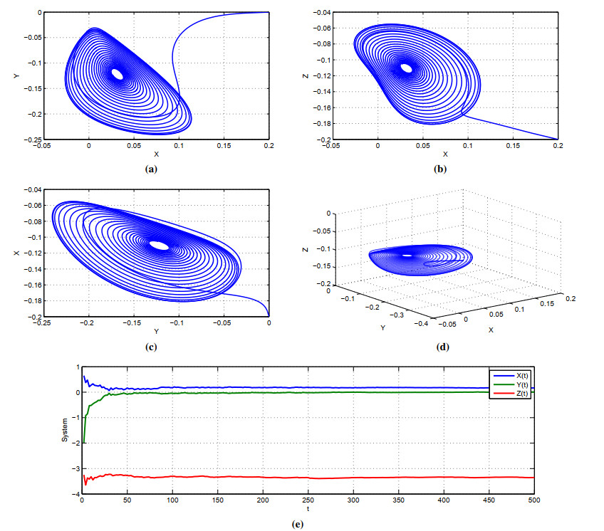
In this work, we formulate a fractal fractional chaotic system with cubic and quadratic nonlinearities. A fractal fractional chaotic Lorenz type and financial systems are studied using the Caputo Fabrizo (CF) fractal fractional derivative. This study focuses on the characterization of the chaotic nature, and the effects of the fractal fractional-order derivative in the CF sense on the evolution and behavior of each proposed systems. The stability of the equilibrium points for the both systems are investigated using the Routh-Hurwitz criterion. The numerical scheme, which includes the discretization of the CF fractal-fractional derivative, is used to depict the phase portraits of the fractal fractional chaotic Lorenz system and the fractal fractional-order financial system. The simulation results presented in both cases include the two- and three-dimensional phase portraits to evaluate the applications of the proposed operators.
- fractal fractional calculus,
- chaotic Lorenz system,
- financial system,
- Routh-Hurwitz stability criterion
Citation: Ihtisham Ul Haq, Shabir Ahmad, Sayed Saifullah, Kamsing Nonlaopon, Ali Akgül. Analysis of fractal fractional Lorenz type and financial chaotic systems with exponential decay kernels[J]. AIMS Mathematics, 2022, 7(10): 18809-18823. doi: 10.3934/math.20221035

Related Papers:

Abstract

In this work, we formulate a fractal fractional chaotic system with cubic and quadratic nonlinearities. A fractal fractional chaotic Lorenz type and financial systems are studied using the Caputo Fabrizo (CF) fractal fractional derivative. This study focuses on the characterization of the chaotic nature, and the effects of the fractal fractional-order derivative in the CF sense on the evolution and behavior of each proposed systems. The stability of the equilibrium points for the both systems are investigated using the Routh-Hurwitz criterion. The numerical scheme, which includes the discretization of the CF fractal-fractional derivative, is used to depict the phase portraits of the fractal fractional chaotic Lorenz system and the fractal fractional-order financial system. The simulation results presented in both cases include the two- and three-dimensional phase portraits to evaluate the applications of the proposed operators.

References

[1]	R. T. Alqahtani, S. Ahmad, A. Akgül, Mathematical analysis of biodegradation model under nonlocal operator in Caputo sense, Mathematics, 9 (2021), 2787. https://doi.org/10.3390/math9212787 doi: 10.3390/math9212787
[2]	M. Arfan, K. Shah, A. Ullah, M. Shutaywi, P. Kumam, Z. Shah, On fractional order model of tumor dynamics with drug interventions under nonlocal fractional derivative, Results Phys., 21 (2021), 103783. https://doi.org/10.1016/j.rinp.2020.103783 doi: 10.1016/j.rinp.2020.103783
[3]	S. Ahmad, A. Ullah, A. Akgül, M. De la Sen, A study of fractional order Ambartsumian equation involving exponential decay kernel, AIMS Math., 6 (2021), 9981–9997. https://doi.org/10.3934/math.2021580 doi: 10.3934/math.2021580
[4]	C. Xu, W. Zhang, C. Aouiti, Z. Liu, M. Liao, P. Li, Further investigation on bifurcation and their control of fractional-order bidirectional associative memory neural networks involving four neurons and multiple delays, Math. Method. Appl. Sci., in press, 2022. https://doi.org/10.1002/mma.7581
[5]	C. Xu, Z. Liu, M. Liao, L. Yao, Theoretical analysis and computer simulations of a fractional order bank data model incorporating two unequal time delays, Expert Syst. Appl., 199 (2022), 116859. https://doi.org/10.1016/j.eswa.2022.116859 doi: 10.1016/j.eswa.2022.116859
[6]	C. Xu, W. Zhang, Z. Liu, P. Li, L. Yao, Bifurcation study for fractional-order three-layer neural networks involving four time delays, Cognit. Comput., 14 (2022), 714–732. https://doi.org/10.1007/s12559-021-09939-1 doi: 10.1007/s12559-021-09939-1
[7]	A. Atangana, Fractal-fractional differentiation and integration: Connecting fractal calculus and fractional calculus to predict complex system, Chaos Soliton. Fract., 102 (2017), 396–406. https://doi.org/10.1016/j.chaos.2017.04.027 doi: 10.1016/j.chaos.2017.04.027
[8]	L. Xuan, S. Ahmad, A. Ullah, S. Saifullah, A. Akgül, H. Qu, Bifurcations, stability analysis and complex dynamics of Caputo fractal-fractional cancer model, Chaos Soliton. Fract., 159 (2022), 112113. https://doi.org/10.1016/j.chaos.2022.112113 doi: 10.1016/j.chaos.2022.112113
[9]	S. Ahmad, A. Ullah, A. Akgül, M. De la Sen, Study of HIV disease and its association with immune cells under nonsingular and nonlocal fractal-fractional operator, Complexity, 2021 (2021), 1904067. https://doi.org/10.1155/2021/1904067 doi: 10.1155/2021/1904067
[10]	A. Akgul, N. Ahmed, A. Raza, Z. Iqbal, M. Rafiq, M. A. Rehman, et al., A fractal fractional model for cervical cancer due to human papillomavirus infection, Fractals, 29 (2021), 2140015. https://doi.org/10.1142/S0218348X21400156 doi: 10.1142/S0218348X21400156
[11]	S. Saifullah, A. Ali, K. Shah, C. Promsakon, Investigation of fractal fractional nonlinear Drinfeld–Sokolov–Wilson system with non-singular operators, Results Phys., 33 (2022), 105145. https://doi.org/10.1016/j.rinp.2021.105145 doi: 10.1016/j.rinp.2021.105145
[12]	A. Atangana, M. A. Khan, Fatmawati, Modeling and analysis of competition model of bank data with fractal-fractional Caputo-Fabrizio operator, Alex. Eng. J., 59 (2020), 1985–1998. https://doi.org/10.1016/j.aej.2019.12.032 doi: 10.1016/j.aej.2019.12.032
[13]	S. Ahmad, A. Ullah, A. Akgül, Investigating the complex behaviour of multi-scroll chaotic system with Caputo fractal-fractional operator, Chaos Soliton. Fract., 146 (2021), 110900. https://doi.org/10.1016/j.chaos.2021.110900 doi: 10.1016/j.chaos.2021.110900
[14]	Z. Ahmad, F. Ali, N. Khan, I. Khan, Dynamics of fractal-fractional model of a new chaotic system of integrated circuit with Mittag-Leffler kernel, Chaos Soliton. Fract., 153 (2021), 111602. https://doi.org/10.1016/j.chaos.2021.111602 doi: 10.1016/j.chaos.2021.111602
[15]	S. Qureshi, A. Atangana, A. A. Shaikh, Strange chaotic attractors under fractal-fractional operators using newly proposed numerical methods, Eur. Phys. J. Plus, 134 (2019), 523. https://doi.org/10.1140/epjp/i2019-13003-7 doi: 10.1140/epjp/i2019-13003-7
[16]	K. A. Abro, A. Atangana, Numerical study and chaotic analysis of meminductor and memcapacitor through fractal-fractional differential operator, Arab. J. Sci. Eng., 46 (2021), 857–871. https://doi.org/10.1007/s13369-020-04780-4 doi: 10.1007/s13369-020-04780-4
[17]	Y. Pan, Nonlinear analysis of a four-dimensional fractional hyper-chaotic system based on general Riemann-Liouville-Caputo fractal-fractional derivative, Nonlinear Dyn., 106 (2021), 3615–3636. https://doi.org/10.1007/s11071-021-06951-w doi: 10.1007/s11071-021-06951-w
[18]	S. Saifullah, A. Ali, E. F. D. Goufo, Investigation of complex behaviour of fractal fractional chaotic attractor with mittag-leffler Kernel, Chaos Soliton. Fract., 152 (2021), 111332. https://doi.org/10.1016/j.chaos.2021.111332 doi: 10.1016/j.chaos.2021.111332
[19]	A. Dlamini, E. F. D. Goufo, M. Khumalo, On the Caputo-Fabrizio fractal fractional representation for the Lorenz chaotic system, AIMS Math., 6 (2021), 12395–12421. https://doi.org/10.5465/AMBPP.2021.12421abstract doi: 10.5465/AMBPP.2021.12421abstract
[20]	S. Sampath, S. Vaidyanathan, Ch. K. Volos, V. T. Pham, An eight-term novel four-scroll chaotic system with cubic nonlinearity and its circuit simulation, J. Eng. Sci. Technol., 8 (2015), 1–6. https://doi.org/10.25103/jestr.082.01 doi: 10.25103/jestr.082.01
[21]	J. H. Ma, Y. S. Chen, Study for the bifurcation topological structure and the global complicated character of a kind of nonlinear finance system (I), Appl. Math. Mech., 22 (2001), 1240–1251. https://doi.org/10.1007/BF02437847 doi: 10.1007/BF02437847

Reader Comments

Your name:*

Email:*
© 2022 the Author(s), licensee AIMS Press. This is an open access article distributed under the terms of the Creative Commons Attribution License (http://creativecommons.org/licenses/by/4.0)