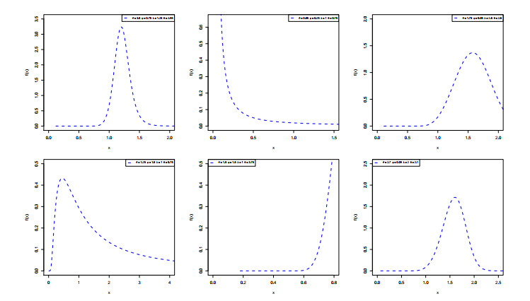
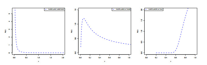
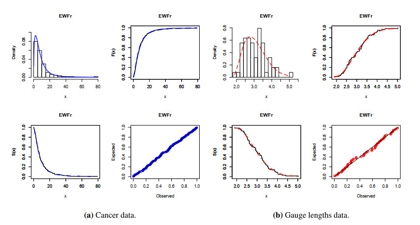
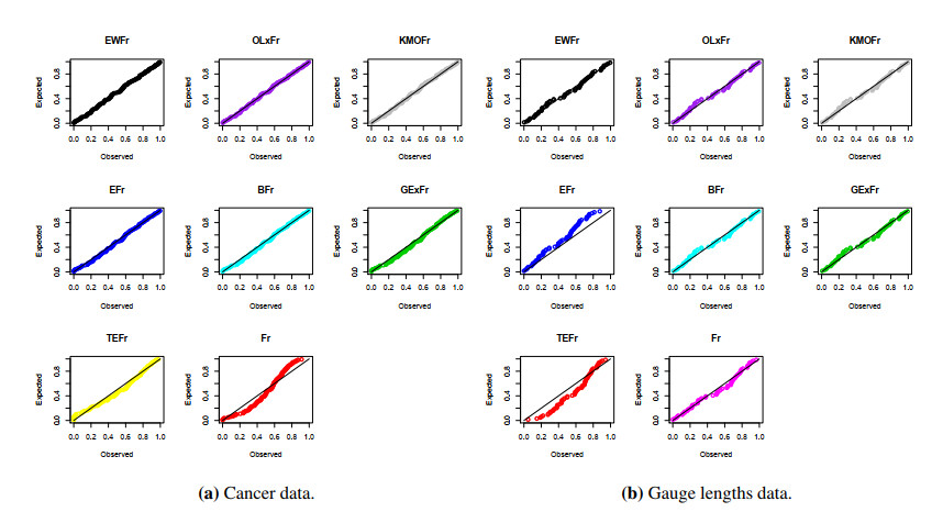
In this paper, a flexible version of the Fréchet distribution called the extended Weibull–Fréchet (EWFr) distribution is proposed. Its failure rate has a decreasing shape, an increasing shape, and an upside-down bathtub shape. Its density function can be a symmetric shape, an asymmetric shape, a reversed-J shape and J shape. Some mathematical properties of the EWFr distribution are explored. The EWFr parameters are estimated using several frequentist estimation approaches. The performance of these methods is addressed using detailed simulations. Furthermore, the best approach for estimating the EWFr parameters is determined based on partial and overall ranks. Finally, the performance of the EWFr distribution is studied using two real-life datasets from the medicine and engineering sciences. The EWFr distribution provides a superior fit over other competing Fréchet distributions such as the exponentiated-Fréchet, beta-Fréchet, Lomax–Fréchet, and Kumaraswamy Marshall–Olkin Fréchet.
Citation: Ekramy A. Hussein, Hassan M. Aljohani, Ahmed Z. Afify. The extended Weibull–Fréchet distribution: properties, inference, and applications in medicine and engineering[J]. AIMS Mathematics, 2022, 7(1): 225-246. doi: 10.3934/math.2022014
In this paper, a flexible version of the Fréchet distribution called the extended Weibull–Fréchet (EWFr) distribution is proposed. Its failure rate has a decreasing shape, an increasing shape, and an upside-down bathtub shape. Its density function can be a symmetric shape, an asymmetric shape, a reversed-J shape and J shape. Some mathematical properties of the EWFr distribution are explored. The EWFr parameters are estimated using several frequentist estimation approaches. The performance of these methods is addressed using detailed simulations. Furthermore, the best approach for estimating the EWFr parameters is determined based on partial and overall ranks. Finally, the performance of the EWFr distribution is studied using two real-life datasets from the medicine and engineering sciences. The EWFr distribution provides a superior fit over other competing Fréchet distributions such as the exponentiated-Fréchet, beta-Fréchet, Lomax–Fréchet, and Kumaraswamy Marshall–Olkin Fréchet.

| [1] |
D. G. Harlow, Applications of the Fréchet distribution function, Int. J. Mater. Prod. Technol., 17 (2002), 482–495. doi: org/10.1504/IJMPT.2002.005472. doi: 10.1504/IJMPT.2002.005472

|
| [2] | S. Kotz, S. Nadarajah, Extreme value distributions: theory and applications, Imperial College Press, London, 2000. doi: org/10.1142/p191. |
| [3] |
M. Mubarak, Parameter estimation based on the Fréchet progressive type II censored data with binomial removals, J. Qual. Statist. Reliab., 2012 (2012), 245910. doi: org/10.1155/2012/245910. doi: 10.1155/2012/245910
|
| [4] |
S. Nadarajah, S. Kotz, Sociological models based on Fréchet random variables, Qual Quant., 42 (2008), 89–95. doi: org/10.1007/s11135-006-9039-1. doi: 10.1007/s11135-006-9039-1
|
| [5] | A. Zaharim, S. K. Najid, A. M. Razali, K. Sopian, Analysing Malaysian wind speed data using statistical distribution, Proceedings of the 4th IASME/WSEAS International Conference on Energy and Environment, Cambridge, 2009. doi: abs/10.5555/1576322.1576388. |
| [6] | S. Nadarajah, S. Kotz, The exponentiated Fréchet distribution, InterStat Electron. J., (2003), 1–7. doi: 10.1.1.529.404&rep=rep1&type=pdf. |
| [7] | S. Nadarajah, A. K. Gupta, The beta Fréchet distribution, Far East J. Theor. Stat., 14 (2004), 15–24. |
| [8] |
E. Krishna, K. K. Jose, T. Alice, M. M. Ristic, The Marshall–Olkin Fréchet distribution, Commun. Stat. Theory Methods, 42 (2013), 4091–4107. doi: org/10.1080/03610926.2011.648785. doi: 10.1080/03610926.2011.648785
|
| [9] |
A. Z. Afify, G. G. Hamedani, I. Ghosh, M. E. Mead, The transmuted Marshall–Olkin Fréchet distribution: Properties and applications, Int. J. Stat. Probab., 4 (2015), 132–184. doi:10.5539/ijsp.v4n4p132. doi: 10.5539/ijsp.v4n4p132
|
| [10] | A. Z. Afify, H. M. Yousof, G. M. Cordeiro, E. M. M. Ortega, Z. M. Nofal, The Weibull Fréchet distribution and its applications. J. Appl. Stat., 43 (2016), 2608–2626. doi: org/10.1080/02664763.2016.1142945. |
| [11] |
M. E. Mead, A. Z. Afify, G. G. Hamedani, I. Ghosh, The beta exponential Fréchet distribution with applications, Austrian J. Stat., 46 (2017), 41–63. doi: 10.17713/ajs.v46i1.144. doi: 10.17713/ajs.v46i1.144
|
| [12] | T. H. M. Abouelmagd, M. S. Hamed, A. Z. Afify, H. Al-Mofleh, Z. Iqbal, The Burr X Fréchet distribution with its properties and applications, J. Appl. Prob. Stat., 13 (2018), 23–51. |
| [13] | M. M. Mansour, E. M. Abd Elrazik, E. Altun, A. Z. Afify, Z. Iqbal, A new three-parameter Fréchet distribution: Properties and applications, Pak. J. Stat., 34 (2018), 441–458. |
| [14] |
A. Afify, A. Shawky, M. Nassar, A new inverse Weibull distribution: Properties, classical and Bayesian estimation with applications, Kuwait J. Sci., 48 (2021), 1–10. doi: org/10.48129/kjs.v48i3.9896. doi: 10.48129/kjs.v48i3.9896
|
| [15] |
M. M. Al Sobhi, The modified Kies–Fréchet distribution: properties, inference and application, AIMS Math., 6 (2021), 4691–4714. doi: 10.3934/math.2021276. doi: 10.3934/math.2021276
|
| [16] |
M. Alizadeh, E. Altun, A. Z. Afify, G. Ozel, The extended odd Weibull-G family: Properties and applications, Commun. Fac. Sci. Univ. Ank. Ser. A1 Math. Stat., 68 (2019), 161–186. doi: org/10.31801/cfsuasmas.443699. doi: 10.31801/cfsuasmas.443699
|
| [17] |
R. A. Maller, S. Zhou, Testing for the presence of immune or cured individuals in censored survival data, Biometrics, 51 (1995), 1197–1205. doi: org/10.2307/2533253. doi: 10.2307/2533253
|
| [18] |
G. C. Perdoná, F. Louzada-Neto, A general hazard model for lifetime data in the presence of cure rate, J. Appl. Stat., 38 (2011), 1395–1405. doi: org/10.1080/02664763.2010.505948. doi: 10.1080/02664763.2010.505948
|
| [19] |
J. J. Swain, S. Venkatraman, J. R. Wilson, Least-squares estimation of distribution functions in johnson's translation system, J. Stat. Comput. Simul., 29 (1988), 271–297. doi: org/10.1080/00949658808811068. doi: 10.1080/00949658808811068
|
| [20] |
A. Luceño, Fitting the generalized pareto distribution to data using maximum goodness-of-fit estimators, Comput. Stat. Data Anal., 51 (2006), 904–917. doi: 10.1016/j.csda.2005.09.011. doi: 10.1016/j.csda.2005.09.011
|
| [21] | R. B. D'Agostino, Goodness-of-fit-techniques, Statistics: A series of textbooks and monographs, Taylor & Francis, 1986. |
| [22] | R Core Team. R: A language and environment for statistical computing, R foundation for statistical computing: Vienna, Austria, 2020. Available online: https://www.R-project.org/. |
| [23] | E. T. Lee, J. W. Wang, Statistical methods for survival data analysis, 3rd ed., John Wiley and Sons, Inc.: Hoboken, NJ, USA, 2003. |
| [24] |
M. R. Alkasasbeh, M. Z. Raqab, Estimation of the generalized logistic distribution parameters: Comparative study, Stat. Method., 6 (2009), 262–279. doi: 10.1016/j.stamet.2008.10.001. doi: 10.1016/j.stamet.2008.10.001
|
| [25] |
M. S. Hamed, F. Aldossary, A. Z. Afify, The four-parameter Fréchet distribution: Properties and applications, Pak. J. Stat. Oper. Res., 16 (2020), 249–264. doi: org/10.18187/pjsor.v16i2.3097. doi: 10.18187/pjsor.v16i2.3097
|
| [26] | A. Z. Afify, H. M. Yousof, G. M. Cordeiro, Z. M. Nofal, M. Ahmad, The Kumaraswamy Marshall–Olkin Fréchet distribution with application, J. ISOSS, 2 (2016), 151–168. |
| [27] |
R. V. D. Silva, T. A. de Andrade, D. Maciel, R. P. Campos, G. M. Cordeiro, A new lifetime model: The gamma extended Fréchet distribution, J. Stat. Theory Appl., 12 (2013), 39–54. doi: org/10.2991/jsta.2013.12.1.4. doi: 10.2991/jsta.2013.12.1.4
|
| [28] |
I. Elbatal, G. Asha, A. V. Raja, Transmuted exponentiated Fréchet distribution: Properties and applications, J. Stat. Appl. Prob., 3 (2014), 379. doi: org/10.12785/jsap/030309. doi: 10.12785/jsap/030309
|
Figures(4) / Tables(11)

Ekramy A. Hussein, Hassan M. Aljohani, Ahmed Z. Afify. The extended Weibull–Fréchet distribution: properties, inference, and applications in medicine and engineering[J]. AIMS Mathematics, 2022, 7(1): 225-246. doi: 10.3934/math.2022014


 DownLoad: