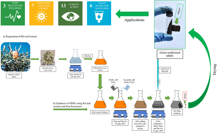
Magnetite nanoparticles (MNPs) were synthesized by a straightforward one-step biogenic process using a leaf extract taken from the Australian indigenous plant Banksia ashbyi (BA). Several advanced characterization techniques, such as X-ray diffraction (XRD), Fourier transform infrared spectroscopy (FT-IR), energy-dispersive spectroscopy (EDS), thermogravimetric analysis (TGA), and Raman spectroscopy were used to investigate the physical and chemical properties of synthesized MNPs. In addition, the size and morphology of the synthesized particles were examined using both focused ion beam scanning electron microscopy (FIBSEM) and transmission electron microscopy (TEM) methods. FT-IR analysis revealed the presence of a Fe–O band located at 551 cm-1, which confirmed the formation of BA-MNPs. Both FIBSEM and TEM image analysis confirmed the nanoparticles were spherical in shape and had a mean diameter of 18 nm with a particle distribution that ranged between 13 and 23 nm. The strong iron (Fe) and oxygen (O) peaks seen in the EDS analysis also confirmed the formation of the MNPs. TGA analysis revealed the leaf extract not only acted as the reducing agent but also served as a capping agent. The XRD analysis revealed that the synthesized MNPs exhibited a high degree of crystallinity and did not contain any impurities. Furthermore, X-ray peak profile analysis using Williamson-Hall methods found the average crystallite size was 9.13 nm, with the crystal lattice experiencing a compressive stress of 546.5 MPa and an average micro-strain of 2.54 × 10⁻³. In addition, other material properties such as density (5.260 kg/m3), average Young's modulus of elasticity (217 GPa), modulus of rigidity (90 GPa), and Poisson's ratio (0.235) were also estimated from the XRD data.
Citation: Gérrard Eddy Jai Poinern, A F M Fahad Halim, Derek Fawcett, Peter Chapman, Rupam Sharma. Banksia Ashbyi-engineered facile green synthesis of magnetite nanoparticles: Characterization, and determination of micro-strain, stress, and physical parameters by X-ray-based Williamson-Hall analysis[J]. AIMS Materials Science, 2024, 11(6): 1096-1124. doi: 10.3934/matersci.2024053
Magnetite nanoparticles (MNPs) were synthesized by a straightforward one-step biogenic process using a leaf extract taken from the Australian indigenous plant Banksia ashbyi (BA). Several advanced characterization techniques, such as X-ray diffraction (XRD), Fourier transform infrared spectroscopy (FT-IR), energy-dispersive spectroscopy (EDS), thermogravimetric analysis (TGA), and Raman spectroscopy were used to investigate the physical and chemical properties of synthesized MNPs. In addition, the size and morphology of the synthesized particles were examined using both focused ion beam scanning electron microscopy (FIBSEM) and transmission electron microscopy (TEM) methods. FT-IR analysis revealed the presence of a Fe–O band located at 551 cm-1, which confirmed the formation of BA-MNPs. Both FIBSEM and TEM image analysis confirmed the nanoparticles were spherical in shape and had a mean diameter of 18 nm with a particle distribution that ranged between 13 and 23 nm. The strong iron (Fe) and oxygen (O) peaks seen in the EDS analysis also confirmed the formation of the MNPs. TGA analysis revealed the leaf extract not only acted as the reducing agent but also served as a capping agent. The XRD analysis revealed that the synthesized MNPs exhibited a high degree of crystallinity and did not contain any impurities. Furthermore, X-ray peak profile analysis using Williamson-Hall methods found the average crystallite size was 9.13 nm, with the crystal lattice experiencing a compressive stress of 546.5 MPa and an average micro-strain of 2.54 × 10⁻³. In addition, other material properties such as density (5.260 kg/m3), average Young's modulus of elasticity (217 GPa), modulus of rigidity (90 GPa), and Poisson's ratio (0.235) were also estimated from the XRD data.

| [1] |
Ahmadi S, Chia CH, Zakaria S, et al. (2012) Synthesis of Fe3O4 nanocrystals using hydrothermal approach. J Magn Magn Mater 324: 4147–4150. https://doi.org/10.1016/j.jmmm.2012.07.023 doi: 10.1016/j.jmmm.2012.07.023

|
| [2] | Montoro VNCE (1938) Miscibilita fra gli ossidi salini di ferro e di manganese. Gaz Chim Ital 68: 728–733. |
| [3] | Cotar AI, Grumezescu AM, Huang KS, et al. (2013) Magnetite nanoparticles influence the efficacy of antibiotics against biofilm embedded Staphylococcus aureus cells. Biointerface Res Appl Chem 3: 559–565. Available from: http://grumezescu.com/?corpo_portfolio = magnetite-nanoparticles-influence-the-efficacy-of-antibiotics-against-biofilm-embeddedstaphylococcus-aureus-cells. |
| [4] |
Gu T, Zhang Y, Khan SA, et al. (2019) Continuous flow synthesis of superparamagnetic nanoparticles in reverse miniemulsion systems. Colloid Interface Sci Commun 28: 1–4. https://doi.org/10.1016/j.colcom.2018.10.005 doi: 10.1016/j.colcom.2018.10.005
|
| [5] |
Ma J, Lee SMY, Yi C, et al. (2017) Controllable synthesis of functional nanoparticles by microfluidic platforms for biomedical applications—A review. Lab Chip 17: 209–226. https://doi.org/10.1039/C6LC01049K doi: 10.1039/C6LC01049K
|
| [6] |
Mohammadi H, Nekobahr E, Akhtari J, et al. (2021) Synthesis and characterization of magnetite nanoparticles by co-precipitation method coated with biocompatible compounds and evaluation of in-vitro cytotoxicity. Toxicol Rep 8: 331–336. https://doi.org/10.1016/j.toxrep.2021.01.012 doi: 10.1016/j.toxrep.2021.01.012
|
| [7] |
Soleymani M, Khalighfard S, Khodayari S, et al. (2020) Effects of multiple injections on the efficacy and cytotoxicity of folate-targeted magnetite nanoparticles as theranostic agents for MRI detection and magnetic hyperthermia therapy of tumor cells. Sci Rep 10: 1695. https://doi.org/10.1038/s41598-020-58605-3 doi: 10.1038/s41598-020-58605-3
|
| [8] |
Chircov C, Grumezescu AM, Holban AM (2019) Magnetic particles for advanced molecular diagnosis. Materials 12: 2158. https://doi.org/10.3390/ma12132158 doi: 10.3390/ma12132158
|
| [9] |
López YC, Antuch M (2020) Morphology control in the plant-mediated synthesis of magnetite nanoparticles. Curr Opin Green Sustainable Chem 24: 32–37. https://doi.org/10.1016/j.cogsc.2020.02.001 doi: 10.1016/j.cogsc.2020.02.001
|
| [10] |
Zhao CX, He L, Qiao SZ, et al. (2011) Nanoparticle synthesis in microreactors. Chem Eng Sci 66: 1463–1479. https://doi.org/10.1016/j.ces.2010.08.039 doi: 10.1016/j.ces.2010.08.039
|
| [11] |
Ficai D, Grumezescu V, Fufă OM, et al. (2018) Antibiofilm coatings based on PLGA and nanostructured cefepime-functionalized magnetite. Nanomaterials 8: 633. https://doi.org/10.3390/nano8090633 doi: 10.3390/nano8090633
|
| [12] |
Sirivat A, Paradee N (2019) Facile synthesis of gelatin-coated Fe3O4 nanoparticle: Effect of pH in single-step co-precipitation for cancer drug loading. Mater Design 181: 107942. https://doi.org/10.1016/j.matdes.2019.107942 doi: 10.1016/j.matdes.2019.107942
|
| [13] | Taufiq A, Nikmah A, Hidayat A, et al. (2020) Synthesis of magnetite/silica nanocomposites from natural sand to create a drug delivery vehicle. Heliyon 6: e03784. https://doi.org/10.1016/j.heliyon.2020.e03784 |
| [14] |
Ladole MR, Pokale PB, Patil SS, et al. (2020) Laccase immobilized peroxidase mimicking magnetic metal organic frameworks for industrial dye degradation. Bioresour Technol 317: 124035. https://doi.org/10.1016/j.biortech.2020.124035 doi: 10.1016/j.biortech.2020.124035
|
| [15] |
De Queiroz DF, de Camargo ER, Martines MU (2020) Synthesis and characterization of magnetic nanoparticles of cobalt ferrite coated with silica. Biointerface Res Appl Chem 10: 4908–4913. https://doi.org/10.33263/BRIAC101.908913 doi: 10.33263/BRIAC101.908913
|
| [16] | Gao G, Liu X, Shi R, et al. (2010) Shape-controlled synthesis and magnetic properties of monodisperse Fe3O4 nanocubes. Crystal Growth Design 10: 2888–2894. https://pubs.acs.org/doi/full/10.1021/cg900920q |
| [17] | Amendola V, Riello P, Meneghetti M (2011) Magnetic nanoparticles of iron carbide, iron oxide, iron@iron oxide, and metal iron synthesized by laser ablation in organic solvents. J Phys Chem C 115: 5140–5146. https://pubs.acs.org/doi/full/10.1021/jp109371m |
| [18] |
Novoselova LY (2021) Nanoscale magnetite: New synthesis approach, structure and properties. Appl Surf Sci 539: 148275. https://doi.org/10.1016/j.apsusc.2020.148275 doi: 10.1016/j.apsusc.2020.148275
|
| [19] |
Kolchanov DS, Slabov V, Keller K, et al. (2019) Sol–gel magnetite inks for inkjet printing. J Mater Chem C 7: 6426–6432. https://doi.org/10.1039/C9TC00311H doi: 10.1039/C9TC00311H
|
| [20] |
Menard MC, Takeuchi KJ, Marschilok AC, et al. (2013) Electrochemical discharge of nanocrystalline magnetite: Structure analysis using X-ray diffraction and X-ray absorption spectroscopy. Phys Chem Chem Phys 15: 18539–18548. https://doi.org/10.1039/C3CP52870G doi: 10.1039/C3CP52870G
|
| [21] |
Zhang S, Li W, Tan B, et al. (2015) One-pot synthesis of ultra-small magnetite nanoparticles on the surface of reduced graphene oxide nanosheets as anodes for sodium-ion batteries. J Mater Chem A 3: 4793–4798. https://doi.org/10.1039/C4TA06708H doi: 10.1039/C4TA06708H
|
| [22] |
Zaidi SDA, Wang C, Gyö rgy B, et al. (2020) Iron and silicon oxide doped/PAN-based carbon nanofibers as free-standing anode material for Li-ion batteries. J Colloid Interface Sci 569: 164–176. https://doi.org/10.1016/j.jcis.2020.02.059 doi: 10.1016/j.jcis.2020.02.059
|
| [23] |
Li J, Li Y, Chen X, et al. (2019) Selective synthesis of magnetite nanospheres with controllable morphologies on CNTs and application to lithium-ion batteries. Phys Status Solidi A 216: 1800924. https://doi.org/10.1002/pssa.201800924 doi: 10.1002/pssa.201800924
|
| [24] |
Sajid M, Płotka-Wasylka J (2020) Nanoparticles: Synthesis, characteristics, and applications in analytical and other sciences. Microchem J 154: 104623. https://doi.org/10.1016/j.microc.2020.104623 doi: 10.1016/j.microc.2020.104623
|
| [25] |
Mohamed G, Hassan N, Shahat A, et al. (2021) Synthesis and characterization of porous magnetite nanosphere iron oxide as a novel adsorbent of anionic dyes removal from aqueous solution. Biointerface Res Appl Chem 11: 13377–13401. https://doi.org/10.33263/BRIAC115.1337713401 doi: 10.33263/BRIAC115.1337713401
|
| [26] |
Masuku M, Ouma L, Pholosi A, et al. (2021) Microwave-assisted synthesis of oleic acid-modified magnetite nanoparticles for benzene adsorption. Environ Nanotechnol Monit Manag 15: 100429. https://doi.org/10.1016/j.enmm.2021.100429 doi: 10.1016/j.enmm.2021.100429
|
| [27] | Jalil MA, Halim AFMF, Moniruzzaman M, et al. (2023) Nano materials in textile processing, In: Rahman MM, Mashud M, Rahman MM, Advanced Technology in Textiles. Textile Science and Clothing Technology, Singapore: Springer Nature. https://doi.org/10.1007/978-981-99-2142-3_12 |
| [28] |
Saif S, Tahir A, Chen Y, et al. (2016) Green synthesis of iron nanoparticles and their environmental applications and implications. Nanomaterials 6: 209. https://doi.org/10.3390/nano6110209 doi: 10.3390/nano6110209
|
| [29] |
Bruschi ML, de Toledo LDAS (2019) Pharmaceutical applications of iron-oxide magnetic nanoparticles. Magnetochemistry 5: 50. https://doi.org/10.3390/magnetochemistry5030050 doi: 10.3390/magnetochemistry5030050
|
| [30] |
Ghazanfari MR, Kashefi M, Shams SF, et al. (2016) Perspective of Fe₃O₄ nanoparticles' role in biomedical applications. Biochem Res Int 2016: 7840161. https://doi.org/10.1155/2016/7840161 doi: 10.1155/2016/7840161
|
| [31] |
Gao G, Shi R, Qin W, et al. (2010) Solvothermal synthesis and characterization of size-controlled monodisperse Fe₃O₄ nanoparticles. J Mater Sci 45: 3483–3489. https://doi.org/10.1007/s10853-010-4378-7 doi: 10.1007/s10853-010-4378-7
|
| [32] |
Satvekar RK, Rohiwal SS, Tiwari AP, et al. (2015) Sol–gel derived silica/chitosan/Fe₃O₄ nanocomposite for direct electrochemistry and hydrogen peroxide biosensing. Mater Res Express 2: 015402. https://doi.org/10.1088/2053-1591/2/1/015402 doi: 10.1088/2053-1591/2/1/015402
|
| [33] |
Manikandan A, Vijaya JJ, Mary JA, et al. (2014) Structural, optical, and magnetic properties of Fe₃O₄ nanoparticles prepared by a facile microwave combustion method. J Ind Eng Chem 20: 2077–2085. https://doi.org/10.1016/j.jiec.2013.09.035 doi: 10.1016/j.jiec.2013.09.035
|
| [34] |
Kalantari K, Ahmad MB, Shameli K, et al. (2013) Synthesis of talc/Fe₃O₄ magnetic nanocomposites using the chemical co-precipitation method. Int J Nanomedicine 8: 1817–1823. https://doi.org/10.2147/IJN.S43693 doi: 10.2147/IJN.S43693
|
| [35] |
Wu S, Sun A, Zhai F, et al. (2011) Fe₃O₄ magnetic nanoparticles synthesis from tailings by ultrasonic chemical co-precipitation. Mater Lett 65: 1882–1884. https://doi.org/10.1016/j.matlet.2011.03.065 doi: 10.1016/j.matlet.2011.03.065
|
| [36] |
Osman AI, Zhang Y, Farghali M, et al. (2024) Synthesis of green nanoparticles for energy, biomedical, environmental, agricultural, and food applications: A review. Environ Chem Lett 22: 841–887. https://doi.org/10.1007/s10311-023-01682-3 doi: 10.1007/s10311-023-01682-3
|
| [37] |
Sánchez-López E, Gomes D, Esteruelas G, et al. (2020) Metal-based nanoparticles as antimicrobial agents: An overview. Nanomaterials 10: 292. https://doi.org/10.3390/nano10020292 doi: 10.3390/nano10020292
|
| [38] | Kumar PSR, Alexis SJ (2019) Synthesized carbon nanotubes and their applications, In: Yaragalla S, Mishra R, Thomas S, et al. Carbon-Based Nanofillers and Their Rubber Nanocomposites, Amsterdam: Elsevier, 109–122. https://doi.org/10.1016/B978-0-12-813248-7.00004-3 |
| [39] |
Singh P, Kim YJ, Zhang D, et al. (2016) Biological synthesis of nanoparticles from plants and microorganisms. Trends Biotechnol 34: 588–599. https://doi.org/10.1016/j.tibtech.2016.02.006 doi: 10.1016/j.tibtech.2016.02.006
|
| [40] |
Mihai AD, Chircov C, Grumezescu AM, et al. (2020) Magnetite nanoparticles and essential oil systems for advanced antibacterial therapies. Int J Mol Sci 21: 7355. https://doi.org/10.3390/ijms21197355 doi: 10.3390/ijms21197355
|
| [41] |
Prabhu NN (2018) Green synthesis of iron oxide nanoparticles (IONPs) and their nanotechnological applications. J Bacteriol Mycol Open Access 6: 260–262. https://doi.org/10.15406/jbmoa.2018.06.00215 doi: 10.15406/jbmoa.2018.06.00215
|
| [42] |
López YC, Antuch M (2020) Morphology control in the plant-mediated synthesis of magnetite nanoparticles. Curr Opin Green Sustainable Chem 24: 32–37. https://doi.org/10.1016/j.cogsc.2020.02.001 doi: 10.1016/j.cogsc.2020.02.001
|
| [43] |
Rathinavel S, Priyadharshini K, Panda D (2021) A review on carbon nanotube: An overview of synthesis, properties, functionalization, characterization, and the application. Mater Sci Eng B 268: 115095. https://doi.org/10.1016/j.mseb.2021.115095 doi: 10.1016/j.mseb.2021.115095
|
| [44] |
Ma Z, Mohapatra J, Wei K, et al. (2021) Magnetic nanoparticles: Synthesis, anisotropy, and applications. Chem Rev 123: 3904–3943. https://doi.org/10.1021/acs.chemrev.1c00860 doi: 10.1021/acs.chemrev.1c00860
|
| [45] |
Rattan S, Derek Fawcett D, Poinern GEJ, et al. (2021) Williamson-Hall-based X-ray peak profile evaluation and nano-structural characterization of rod-shaped hydroxyapatite powder for potential dental restorative procedures. AIMS Mater Sci 8: 359–372. https://doi.org/10.3934/matersci.2021023 doi: 10.3934/matersci.2021023
|
| [46] |
Ayeshamariam A, Sanjeeviraja C, Jayachandran M, et al. (2011) Synthesization, characterization, and gas sensing properties of SnO₂ nanoparticles. Int J Chem Anal Sci 2: 54–61. https://doi.org/10.1166/jno.2013.1471 doi: 10.1166/jno.2013.1471
|
| [47] |
Cullity BD, Smoluchowski R (1957) Elements of X‐ray diffraction. Phys Today 10: 50. https://doi.org/10.1063/1.3060306 doi: 10.1063/1.3060306
|
| [48] |
Aly KA, Khalil NM, Algamal Y, et al. (2016) Lattice strain estimation for CoAl₂O₄ nanoparticles using Williamson-Hall analysis. J Alloys Compd 676: 606–612. https://doi.org/10.1016/j.jallcom.2016.03.213 doi: 10.1016/j.jallcom.2016.03.213
|
| [49] |
Harjo S, Tomota Y, Torii S, et al. (2002) Residual thermal phase stresses in α–γ Fe–Cr–Ni alloys measured by a neutron diffraction time-of-flight method. Mater Trans 43: 1696–1702. https://doi.org/10.2320/matertrans.43.1696 doi: 10.2320/matertrans.43.1696
|
| [50] |
Biju V, Sugathan N, Vrinda V, et al. (2008) Estimation of lattice strain in nanocrystalline silver from X-ray diffraction line broadening. J Mater Sci 43: 1175–1179. https://doi.org/10.1007/s10853-007-2300-8 doi: 10.1007/s10853-007-2300-8
|
| [51] |
Ravinder D, Alivelumanga T (1998) Composition dependence of elastic behaviour of mixed manganese–zinc ferrites. Mater Lett 37: 51–56. https://doi.org/10.1016/S0167-577X(98)00062-7 doi: 10.1016/S0167-577X(98)00062-7
|
| [52] |
Yusefi M, Shameli K, Ali RR, et al. (2020) Evaluating anticancer activity of plant-mediated synthesized iron oxide nanoparticles using Punica granatum fruit peel extract. J Mol Struct 1204: 127539. https://doi.org/10.1016/j.molstruc.2019.127539 doi: 10.1016/j.molstruc.2019.127539
|
| [53] |
Izadiyan Z, Shameli K, Miyake M, et al. (2020) Cytotoxicity assay of plant-mediated synthesized iron oxide nanoparticles using Juglans regia green husk extract. Arab J Chem 13: 2011–2023. https://doi.org/10.1016/j.arabjc.2018.02.019 doi: 10.1016/j.arabjc.2018.02.019
|
| [54] |
Hearmon RFS (1956) The elastic constants of anisotropic materials—Ⅱ. Adv Phys 5: 323–382. https://doi.org/10.1080/00018732.1956.tADP0323 doi: 10.1080/00018732.1956.tADP0323
|
| [55] |
Chaki SH, Malek TJ, Chaudhary MD, et al. (2015) Magnetite Fe3O4 nanoparticles synthesis by wet chemical reduction and their characterization. Adv Nat Sci Nanosci Nanotechnol 6: 035009. https://doi.org/10.1088/2043-6262/6/3/035009 doi: 10.1088/2043-6262/6/3/035009
|
| [56] |
Yusoff AHM, Salimi MN, Jamlos MF (2017) Dependence of lattice strain of magnetite nanoparticles on precipitation temperature and pH of solution. J Phys Conf Ser 908: 012065. https://doi.org/10.1088/1742-6596/908/1/012065 doi: 10.1088/1742-6596/908/1/012065
|
| [57] |
Kushwaha P, Chauhan P (2021) Microstructural evaluation of iron oxide nanoparticles at different calcination temperature by Scherrer, Williamson-Hall, Size-Strain Plot and Halder-Wagner methods. Phase Transit 94: 731–753. https://doi.org/10.1080/01411594.2021.1969396 doi: 10.1080/01411594.2021.1969396
|
| [58] |
Ilyas S, Abdullah B, Tahir D (2019) X-ray diffraction analysis of nanocomposite Fe3O4/activated carbon by Williamson-Hall and size-strain plot methods. Nano Struct Nano Objects 20: 100396. https://doi.org/10.1016/j.nanoso.2019.100396 doi: 10.1016/j.nanoso.2019.100396
|
| [59] |
Yusefi M, Shameli K, Ali RR, et al. (2020) Evaluating anticancer activity of plant-mediated synthesized iron oxide nanoparticles using Punica granatum fruit peel extract. J Mol Struct 1204: 127539. https://doi.org/10.1016/j.molstruc.2019.127539 doi: 10.1016/j.molstruc.2019.127539
|
| [60] |
Vives S, Gaffet E, Meunier C (2004) X-ray diffraction line profile analysis of iron ball milled powders. Mater Sci Eng A 366: 229–238. https://doi.org/10.1016/S0921-5093(03)00572-0 doi: 10.1016/S0921-5093(03)00572-0
|
| [61] |
Jafari A, Farjami Shayesteh S, Salouti M, et al. (2015) Dependence of structural phase transition and lattice strain of Fe3O4 nanoparticles on calcination temperature. Indian J Phys 89: 551–560. https://doi.org/10.1007/s12648-014-0627-y doi: 10.1007/s12648-014-0627-y
|
| [62] |
Zak AK, Majid WA, Abrishami ME, et al. (2011) X-ray analysis of ZnO nanoparticles by Williamson-Hall and size–strain plot methods. Solid State Sci 13: 251–256. https://doi.org/10.1016/j.solidstatesciences.2010.11.024 doi: 10.1016/j.solidstatesciences.2010.11.024
|
| [63] |
Rana G, Johri UC (2014) Correlation between the pH value and properties of magnetite nanoparticles. Adv Mater Lett 5: 280–286. https://doi.org/10.5185/amlett.2014.10563 doi: 10.5185/amlett.2014.10563
|
| [64] |
Gholizadeh A (2017) A comparative study of physical properties in Fe3O4 nanoparticles prepared by coprecipitation and citrate methods. J Am Ceram Soc 100: 3577–3588. https://doi.org/10.1111/jace.14896 doi: 10.1111/jace.14896
|
| [65] |
Suppiah DD, Abd Hamid SB (2016) One step facile synthesis of ferromagnetic magnetite nanoparticles. J Magn Magn Mater 414: 204–208. https://doi.org/10.1016/j.jmmm.2016.04.072 doi: 10.1016/j.jmmm.2016.04.072
|
| [66] |
Da'na E, Taha A, Afkar E (2018) Green synthesis of iron nanoparticles by Acacia nilotica pods extract and its catalytic, adsorption, and antibacterial activities. Appl Sci 8: 1922. https://doi.org/10.3390/app8101922 doi: 10.3390/app8101922
|
| [67] |
Van Ommen JR, Valverde JM, Pfeffer R (2012) Fluidization of nanopowders: A review. J Nanopart Res 14: 1–29. https://doi.org/10.1007/s11051-012-0737-4 doi: 10.1007/s11051-012-0737-4
|
| [68] |
Bassim S, Mageed AK, AbdulRazak AA, et al. (2022) Green synthesis of Fe3O4 nanoparticles and its applications in wastewater treatment. Inorganics 10: 260. https://doi.org/10.3390/inorganics10120260 doi: 10.3390/inorganics10120260
|
| [69] |
Wei R, Li H, Lin Y, et al. (2020) Reduction characteristics of iron oxide by the hemicellulose, cellulose, and lignin components of biomass. Energy Fuels 34: 8332–8339. https://doi.org/10.1021/acs.energyfuels.0c00377 doi: 10.1021/acs.energyfuels.0c00377
|
| [70] |
Laid TM, Abdelhamid K, Eddine LS, et al. (2021) Optimizing the biosynthesis parameters of iron oxide nanoparticles using central composite design. J Mol Struct 1229: 129497. https://doi.org/10.1016/j.molstruc.2020.129497 doi: 10.1016/j.molstruc.2020.129497
|
| [71] |
Anukam AI, Berghel J, Famewo EB, et al. (2020) Improving the understanding of the bonding mechanism of primary components of biomass pellets through the use of advanced analytical instruments. J Wood Chem Technol 40: 15–32. https://doi.org/10.1080/02773813.2019.1652324 doi: 10.1080/02773813.2019.1652324
|
| [72] |
Ramesh AV, Rama Devi D, Mohan Botsa S, et al. (2018) Facile green synthesis of Fe3O4 nanoparticles using aqueous leaf extract of Zanthoxylum armatum DC. for efficient adsorption of methylene blue. J Asian Ceram Soc 6: 145–155. https://doi.org/10.1080/21870764.2018.1459335 doi: 10.1080/21870764.2018.1459335
|
| [73] |
Netala VR, Kotakadi VS, Nagam V, et al. (2015) First report of biomimetic synthesis of silver nanoparticles using aqueous callus extract of Centella asiatica and their antimicrobial activity. Appl Nanosci 5: 801–807. https://doi.org/10.1007/s13204-014-0374-6 doi: 10.1007/s13204-014-0374-6
|
| [74] |
Awwad AM, Salem NM (2012) A green and facile approach for synthesis of magnetite nanoparticles. Nanoscience Nanotechnol 2: 208–213. https://doi.org/10.5923/j.nn.20120206.09 doi: 10.5923/j.nn.20120206.09
|
| [75] |
Arokiyaraj S, Saravanan M, Prakash NU, et al. (2013) Enhanced antibacterial activity of iron oxide magnetic nanoparticles treated with Argemone mexicana L. leaf extract: An in vitro study. Mater Res Bull 48: 3323–3327. https://doi.org/10.1016/j.materresbull.2013.05.059 doi: 10.1016/j.materresbull.2013.05.059
|
| [76] |
Rahmani R, Gharanfoli M, Gholamin M, et al. (2020) Plant-mediated synthesis of superparamagnetic iron oxide nanoparticles (SPIONs) using aloe vera and flaxseed extracts and evaluation of their cellular toxicities. Ceram Int 46: 3051–3058. https://doi.org/10.1016/j.ceramint.2019.10.005 doi: 10.1016/j.ceramint.2019.10.005
|
| [77] |
Rahmayanti M, Syakina AN, Fatimah I, et al. (2022) Green synthesis of magnetite nanoparticles using peel extract of jengkol (Archidendron pauciflorum) for methylene blue adsorption from aqueous media. Chem Phys Lett 803: 139834. https://doi.org/10.1016/j.cplett.2022.139834 doi: 10.1016/j.cplett.2022.139834
|
| [78] |
Ghoohestani E, Samari F, Homaei A, et al. (2024) A facile strategy for preparation of Fe₃O₄ magnetic nanoparticles using Cordia myxa leaf extract and investigating its adsorption activity in dye removal. Sci Rep 14: 84. https://doi.org/10.1038/s41598-023-50550-1 doi: 10.1038/s41598-023-50550-1
|
| [79] |
Hasan K, Shehadi IA, Al-Bab ND, et al. (2019) Magnetic chitosan-supported silver nanoparticles: A heterogeneous catalyst for the reduction of 4-nitrophenol. Catalysts 9: 839. https://doi.org/10.3390/catal9100839 doi: 10.3390/catal9100839
|
| [80] | Halim AF, Poinern GE, Fawcett D, et al. (2024) Green biogenic synthesis of magnetite nanoparticles from indigenous Banksia ashbyi leaf for enhanced sonochemical dye degradation. Mater Res Express. https://doi.org/10.1088/2053-1591/ad8ca0 |
| [81] |
Yusefi M, Shameli K, Yee OS, et al. (2021) Green synthesis of Fe3O4 nanoparticles stabilized by a Garcinia mangostana fruit peel extract for hyperthermia and anticancer activities. Int J Nanomed 16: 2515. https://doi.org/10.2147/IJN.S284134 doi: 10.2147/IJN.S284134
|
| [82] |
Yuvakkumar R, Hong SI (2014) Green synthesis of spinel magnetite iron oxide nanoparticles. Adv Mater Res 1051: 39–42. https://doi.org/10.4028/www.scientific.net/AMR.1051.39 doi: 10.4028/www.scientific.net/AMR.1051.39
|
| [83] |
Murugappan K, Silvester DS, Chaudhary D, et al. (2014) Electrochemical characterization of an oleyl-coated magnetite nanoparticle-modified electrode. ChemElectroChem 1: 1211–1218. https://doi.org/10.1002/celc.201402012 doi: 10.1002/celc.201402012
|
| [84] |
Mishra AK, Ramaprabhu S (2011) Nano magnetite decorated multiwalled carbon nanotubes: A robust nanomaterial for enhanced carbon dioxide adsorption. Energy Environ Sci 4: 889–895. https://doi.org/10.1039/C0EE00076K doi: 10.1039/C0EE00076K
|
| [85] |
Konon M, Brazovskaya EY, Kreisberg V, et al. (2023) Novel inorganic membranes based on magnetite-containing silica porous glasses for ultrafiltration: Structure and sorption properties. Membranes 13: 341. https://doi.org/10.3390/membranes13030341 doi: 10.3390/membranes13030341
|
| [86] |
Taha AB, Essa MS, Chiad BT (2023) Iron oxide nanoparticles preparation by using homemade hydrothermal pyrolysis technique with different reaction times. J Metastable Nanocryst Mater 35: 1–10. https://doi.org/10.4028/p-cbng1t doi: 10.4028/p-cbng1t
|
| [87] |
Sheng-Nana S, Chaoa W, Zan-Zanb Z, et al. (2014) Magnetic iron oxide nanoparticles: Synthesis and surface coating techniques for biomedical applications. Chin Phys B 23: 037503–037519. https://doi.org/10.1088/1674-1056/23/3/037503 doi: 10.1088/1674-1056/23/3/037503
|
| [88] |
Yew YP, Shameli K, Miyake M, et al. (2016) Green synthesis of magnetite (Fe3O4) nanoparticles using seaweed (Kappaphycus alvarezii) extract. Nanoscale Res Lett 11: 1–7. https://doi.org/10.1186/s11671-016-1498-2 doi: 10.1186/s11671-016-1498-2
|
| [89] |
Das C, Sen S, Singh T, et al. (2020) Green synthesis, characterization, and application of natural product coated magnetite nanoparticles for wastewater treatment. Nanomaterials 10: 1615. https://doi.org/10.3390/nano10081615 doi: 10.3390/nano10081615
|
| [90] |
Basavegowda N, Magar KBS, Mishra K, et al. (2014) Green fabrication of ferromagnetic Fe3O4 nanoparticles and their novel catalytic applications for the synthesis of biologically interesting benzoxazinone and benzthioxazinone derivatives. New J Chem 38: 5415–5420. https://doi.org/10.1039/C4NJ01155D doi: 10.1039/C4NJ01155D
|
| [91] |
Basavegowda N, Mishra K, Lee YR (2014) Sonochemically synthesized ferromagnetic Fe3O4 nanoparticles as a recyclable catalyst for the preparation of pyrrolo[3, 4-c]quinoline-1, 3-dione derivatives. RSC Adv 4: 61660–61666. https://doi.org/10.1039/C4RA11623B doi: 10.1039/C4RA11623B
|
| [92] |
Afzal S, Khan R, Zeb T, et al. (2018) Structural, optical, dielectric, and magnetic properties of PVP coated magnetite (Fe3O4) nanoparticles. J Mater Sci Mater Electron 29: 20040–20050. https://doi.org/10.1007/s10854-018-0134-6 doi: 10.1007/s10854-018-0134-6
|
| [93] |
Khan R, Rahman MU, Iqbal Z (2016) Variation of structural, dielectric, and magnetic properties of PVP coated γ-Fe2O3 nanoparticles. J Mater Sci Mater Electron 27: 12490–12498. https://doi.org/10.1007/s10854-016-5634-7 doi: 10.1007/s10854-016-5634-7
|
| [94] |
Mirza I, Sarfraz A, Hasanain S (2014) Effect of surfactant on magnetic and optical properties of α-Fe2O3 nanoparticles. Acta Phys Pol A 126: 1280–1287. https://doi.org/10.12693/APhysPolA.126.1280 doi: 10.12693/APhysPolA.126.1280
|
| [95] |
Attallah OA, Al-Ghobashy MA, Nebsen M, et al. (2018) Assessment of pectin-coated magnetite nanoparticles in low-energy water desalination applications. Environ Sci Pollut Res 25: 18476–18483. https://doi.org/10.1007/s11356-018-2060-9 doi: 10.1007/s11356-018-2060-9
|
| [96] |
Basavaiah K, Kahsay MH, Rama Devi D (2018) Green synthesis of magnetite nanoparticles using aqueous pod extract of Dolichos lablab L for efficient adsorption of crystal violet. Emergent Mater 1: 121–132. https://doi.org/10.1007/s42247-018-0005-1 doi: 10.1007/s42247-018-0005-1
|
| [97] |
Awwad AM, Salem NM (2012) A green and facile approach for synthesis of magnetite nanoparticles. Nanosc Nanotechnol 2: 208–213. https://doi.org/10.5923/j.nn.20120206.09 doi: 10.5923/j.nn.20120206.09
|
| [98] | ISO 14040: 2006. Environmental management-Life cycle assessment-Principles and framework. Available from: https://www.iso.org/standard/37456.html (accessed August 25, 2021). |
| [99] | ISO 14044: 2006. Environmental management-Life cycle assessment-Requirements and guidelines. Available from: https://www.iso.org/standard/38498.html (accessed August 25, 2021). |
| [100] | Al-Hazeef MS, Aidi A, Hecini L, et al. (2024) Valorizing date palm spikelets into activated carbon-derived composite for methyl orange adsorption: Advancing circular bio-economy in wastewater treatment—A comprehensive study on its equilibrium, kinetics, thermodynamics, and mechanisms. Environ Sci Pollut Res 1–20. https://doi.org/10.1007/s11356-024-34581-3 |


Figures(7) / Tables(11)

Gérrard Eddy Jai Poinern, A F M Fahad Halim, Derek Fawcett, Peter Chapman, Rupam Sharma. Banksia Ashbyi-engineered facile green synthesis of magnetite nanoparticles: Characterization, and determination of micro-strain, stress, and physical parameters by X-ray-based Williamson-Hall analysis[J]. AIMS Materials Science, 2024, 11(6): 1096-1124. doi: 10.3934/matersci.2024053


 DownLoad: