Biochemistry tuned by nanopillars

Sumaiya F. Begum; Hai-Feng Ji; Sumaiya F. Begum; Hai-Feng Ji

doi:10.3934/matersci.2021045

AIMS Materials Science

2021, Volume 8, Issue 5: 748-759. doi: 10.3934/matersci.2021045

Previous Article Next Article

Mini review Topical Sections

Biochemistry tuned by nanopillars

Sumaiya F. Begum ,
Hai-Feng Ji ^,

Department of Chemistry, Drexel University, Philadelphia, PA 19104, USA

Received: 04 August 2021 Accepted: 24 September 2021 Published: 29 September 2021

Surface engineering using nanopillars has been used for the fabrication of antimicrobial surfaces, cell culture environments that mimic the extracellular environment, and biosensors for the characterization of biomolecules. In this mini review, we summarize the roles of surface topography on various biochemical processes played by tunable nanopillars.
- biochemistry,
- nanopillars,
- surface topography
Citation: Sumaiya F. Begum, Hai-Feng Ji. Biochemistry tuned by nanopillars[J]. AIMS Materials Science, 2021, 8(5): 748-759. doi: 10.3934/matersci.2021045

Related Papers:

Abstract

Surface engineering using nanopillars has been used for the fabrication of antimicrobial surfaces, cell culture environments that mimic the extracellular environment, and biosensors for the characterization of biomolecules. In this mini review, we summarize the roles of surface topography on various biochemical processes played by tunable nanopillars.

References

[1]	Wang EC, Wang AZ (2014) Nanoparticles and their applications in cell and molecular biology. Integr Biol 6: 9-26. doi: 10.1039/c3ib40165k
[2]	Sathiyamoorthi P, Kim HS (2019) Nanocrystalline high entropy alloys: Processing and properties, Encyclopedia of Materials: Metals and Alloys, Elsevier, 372-380.
[3]	Llor C, Bjerrum L (2014) Antimicrobial resistance: risk associated with antibiotic overuse and initiatives to reduce the problem. Ther Adv Drug Saf 5: 229-241. doi: 10.1177/2042098614554919
[4]	Joerger RD (2003) Alternatives to antibiotics: bacteriocins, antimicrobial peptides and bacteriophages. Poultry Sci 82: 640-647. doi: 10.1093/ps/82.4.640
[5]	Hergt R, Hiergeist R, Hilger I, et al. (2004) Maghemite nanoparticles with very high AC-losses for application in RF-magnetic hyperthermia. J Magn Magn Mater 270: 345-357. doi: 10.1016/j.jmmm.2003.09.001
[6]	Gupta AK, Gupta M (2005) Synthesis and surface engineering of iron oxide nanoparticles for biomedical applications. Biomaterials 26: 3995-4021. doi: 10.1016/j.biomaterials.2004.10.012
[7]	Liu G, Gao J, Ai H, et al. (2013) Applications and potential toxicity of magnetic iron oxide nanoparticles. Small 9: 1533-1545. doi: 10.1002/smll.201201531
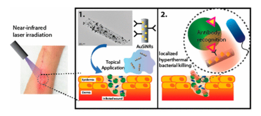
[8]	Alhmoud H, Cifuentes-Rius A, Delalat B, et al. (2017) Gold-decorated porous silicon nanopillars for targeted hyperthermal treatment of bacterial infections. ACS Appl Mater Interf 9: 33707-33716.
[9]	Bandara CD, Singh S, Afara IO, et al. (2017) Bactericidal effects of natural nanotopography of dragonfly wing on Escherichia coli. ACS Appl Mater Interf 9: 6746-6760. doi: 10.1021/acsami.6b13666
[10]	Sugnaux M, Fischer F (2016) Biofilm vivacity and destruction on antimicrobial nanosurfaces assayed within a microbial fuel cell. Nanomed-Nanotechnol 12: 1471-1477. doi: 10.1016/j.nano.2016.03.008
[11]	Pang X, Bian H, Wang W, et al. (2017) A bio-chemical application of N-GQDs and g-C3N4 QDs sensitized TiO₂ nanopillars for the quantitative detection of pcDNA3-HBV. Biosens Bioelectron 91: 456-464. doi: 10.1016/j.bios.2016.12.059
[12]	Migliorini E, Grenci G, Ban J, et al. (2011) Acceleration of neuronal precursors differentiation induced by substrate nanotopography. Biotechol Bioeng 108: 2736-2746. doi: 10.1002/bit.23232
[13]	Brammer KS, Choi C, Frandsen CJ, et al. (2011) Hydrophobic nanopillars initiate mesenchymal stem cell aggregation and osteo-differentiation. Acta Biomater 7: 683-90. doi: 10.1016/j.actbio.2010.09.022
[14]	Koo S, Muhammad R, Peh GS, et al. (2014) Micro-and nanotopography with extracellular matrix coating modulate human corneal endothelial cell behavior. Acta Biomater 10: 1975-1984. doi: 10.1016/j.actbio.2014.01.015
[15]	Wang K, Dang W, Xi D, et al. (2011) Hybridised functional micro-and nanostructure for studying the kinetics of a single biomolecule. Micro Nano Lett 6: 292-295. doi: 10.1049/mnl.2010.0215
[16]	Chen G, McCarley RL, Soper SA, et al. (2007) Functional template-derived poly(methyl methacrylate) nanopillars for solid-phase biological reactions. Chem Mater 19: 3855-3857. doi: 10.1021/cm0702870

Reader Comments

Your name:*

Email:*
© 2021 the Author(s), licensee AIMS Press. This is an open access article distributed under the terms of the Creative Commons Attribution License (http://creativecommons.org/licenses/by/4.0)