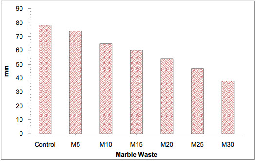
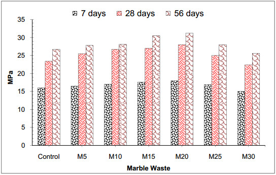
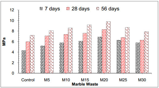
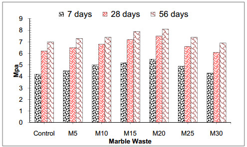
Industrial waste has been rapidly increased day by day because of the fast-expanding population which inappropriately dumps the waste resulting in environmental pollutions. It has been recommended that the disposal of industrial waste would be greatly reduced if it could be incorporated into concrete production. The basic objective of this investigation is to examine the characteristics of concrete using marble slurry as binding material in proportions 5%, 10%, 15%, 20%, 25%, and 30% by weight of cement. Many properties have been reviewed in the current paper; the results observed from the various studies depict that replacement of marble slurry to a certain extent enhances strength properties of the concrete but simultaneously decreases the slump value with the increase of replacement level of marble slurry.
Citation: Jawad Ahmad, Osama Zaid, Muhammad Shahzaib, Muhammad Usman Abdullah, Asmat Ullah, Rahat Ullah. Mechanical properties of sustainable concrete modified by adding marble slurry as cement substitution[J]. AIMS Materials Science, 2021, 8(3): 343-358. doi: 10.3934/matersci.2021022
Industrial waste has been rapidly increased day by day because of the fast-expanding population which inappropriately dumps the waste resulting in environmental pollutions. It has been recommended that the disposal of industrial waste would be greatly reduced if it could be incorporated into concrete production. The basic objective of this investigation is to examine the characteristics of concrete using marble slurry as binding material in proportions 5%, 10%, 15%, 20%, 25%, and 30% by weight of cement. Many properties have been reviewed in the current paper; the results observed from the various studies depict that replacement of marble slurry to a certain extent enhances strength properties of the concrete but simultaneously decreases the slump value with the increase of replacement level of marble slurry.

| [1] |
Agrawal D, Hinge P, Waghe UP, et al. (2014) Utilization of industrial waste in construction material—A review. IJIRSET 3: 8390-8397. doi: 10.15680/IJIRSET.2014.0308073

|
| [2] | Saikia N, Brito J (2009) Use of industrial waste and municipality solid waste as aggregate, filler or fiber in cement mortar and concrete. Adv Mater Sci Res 3: 65-116. |
| [3] |
Li LG, Ouyang Y, Zhuo ZY, et al. (2021) Adding ceramic polishing waste as filler to reduce paste volume and improve carbonation and water resistances of mortar. ABE 2: 1-19. doi: 10.1186/s43251-020-00022-7
|
| [4] |
Ahmad J, Manan A, Ali A, et al. (2020) A study on mechanical and durability aspects of concrete modified with steel fibers (SFs). Civil Eng Archit 8: 814-823. doi: 10.13189/cea.2020.080508
|
| [5] |
Ahmad J, Tufail RF, Aslam F, et al. (2021) A step towards sustainable self-compacting concrete by using partial substitution of wheat straw ash and bentonite clay instead of cement. Sustainability 13: 824. doi: 10.3390/su13020824
|
| [6] |
Bederina M, Makhloufi Z, Bounoua A, et al. (2013) Effect of partial and total replacement of siliceous river sand with limestone crushed sand on the durability of mortars exposed to chemical solutions. Constr Build Mater 47: 146-158. doi: 10.1016/j.conbuildmat.2013.05.037
|
| [7] |
Li LG, Feng JJ, Zhu J, et al. (2021) Pervious concrete: Effects of porosity on permeability and strength. Mag Concrete Res 73: 69-79. doi: 10.1680/jmacr.19.00194
|
| [8] |
Li LG, Huang ZH, Tan YP, et al. (2019) Recycling of marble dust as paste replacement for improving strength, microstructure and eco-friendliness of mortar. J Clean Prod 210: 55-65. doi: 10.1016/j.jclepro.2018.10.332
|
| [9] | Kuswah RP, Sharma IC, Chaurasia PBL (2015) Utilization of marble slurry in cement concrete replacing fine aggregate. AJER 4: 55-58. |
| [10] | Ahmad J, Al-Dala'ien RNS, Manan A, et al. (2020) Evaluating the effects of flexure cracking behaviour of beam reinforced with steel fibres from environment affect. JGE 10: 4998-5016. |
| [11] |
Ahmad J, Aslam F, Zaid O, et al. (2021) Self-fibers compacting concreteproperties reinforced with propylene fibers. Sci Eng Compos Mater 28: 64-72. doi: 10.1515/secm-2021-0006
|
| [12] | El Haggar S (2010) Sustainable Industrial Design and Waste Management: Cradle-to-Cradle for Sustainable Development, Elsevier Academic Press. |
| [13] |
Corinaldesi V, Moriconi G, Naik TR (2010) Characterization of marble powder for its use in mortar and concrete. Constr Build Mater 24: 113-117. doi: 10.1016/j.conbuildmat.2009.08.013
|
| [14] |
Karaşahin M, Terzi S (2007) Evaluation of marble waste dust in the mixture of asphaltic concrete. Constr Build Mater 21: 616-620. doi: 10.1016/j.conbuildmat.2005.12.001
|
| [15] |
Dosho Y (2007) Development of a sustainable concrete waste recycling system. J Adv Concr Technol 5: 27-42. doi: 10.3151/jact.5.27
|
| [16] | Shirulea PA, Rahmanb A, Gupta RD (2012) Partial replacement of cement with marble dust powder. IJAERS 1: 175-177. |
| [17] | Katuwal K, Duarah A, Sarma MK, et al. (2017) Comparative study of M35 concrete using marble dust as partial replacement of cement and fine aggregate. IJIRSET 6: 9094-9100. |
| [18] | Latha G, Reddy AS, Mounika K (2015) Experimental investigation on strength characteristics of concrete using waste marble powder as cementitious material. IJIRSET 4: 12691-12698. |
| [19] | Vigneshpandian GV, Shruthi EA, Venkatasubramanian C, et al. (2017) Utilisation of waste marble dust as fine aggregate in concrete, IOP Conference Series: Earth and Environmental Science, IOP Publishing, 12007. |
| [20] | Kore SD, Vyas AK (2016) Impact of marble waste as coarse aggregate on properties of lean cement concrete. Case Stud Constr Mater 4: 85-92. |
| [21] | Ahmad J, Rehman SU, Zaid O, et al. (2020) To study the characteristics of concrete by using high range water reducing admixture. IJMPERD 10: 14271-14278. |
| [22] | Grout G, ASTM C476, except with a maximum slump of 4 inches, as measured according to ASTM C 143. Available from: https://scholar.google.com/scholar?hl=en&as_sdt=0%2C5&q=22.%09Grout+F+ASTM+C+476%2C+except+with+a+maximum+slump+of+4+inches%2C+as+measured+according+to+ASTM+C+143.+C+143M&btnG=. |
| [23] | ASTM C39/C39M-12a (2012) Standard Test Method for Compressive Strength of Cylindrical Concrete Specimens. |
| [24] |
Shannag MJ, Brincker R, Hansen W (1997) Pullout behavior of steel fibers from cement-based composites. Cement Concrete Res 27: 925-936. doi: 10.1016/S0008-8846(97)00061-6
|
| [25] | Test CC, DrilledT, Concrete C (2010) Standard Test Method for Flexural Strength of Concrete (Using Simple Beam with Third-Point Loading) 1. |
| [26] | Specimen Compression Test, ASTM C31; one set of four standard cylinders for each compressive-strength test, unless otherwise directed. Mold and store cylinders for laboratory-cured test specimens except when field-cured test specimens are required. Available from: https://scholar.google.com/scholar?hl=en&as_sdt=0%2C5&q=26.%09Specimen+CT+ASTM+C+31%3B+one+set+of+four+standard+cylinders+for+each+compressive-strength+test%2C+unless+otherwise+directed.+Mold+store+Cylind+Lab+test+specimens+Except+when+field-cured+test+specimens+are+required&btnG=. |
| [27] |
Aggarwal Y, Siddique R (2014) Microstructure and properties of concrete using bottom ash and waste foundry sand as partial replacement of fine aggregates. Constr Build Mater 54:210-223 doi: 10.1016/j.conbuildmat.2013.12.051
|
| [28] |
Hebhoub H, Aoun H, Belachia M, et al. (2011) Use of waste marble aggregates in concrete. Constr Build Mater 25: 1167-1171. doi: 10.1016/j.conbuildmat.2010.09.037
|
| [29] |
Hameed MS, Sekar ASS, Saraswathy V (2012) Strength and permeability characteristics study of self-compacting concrete using crusher rock dust and marble sludge powder. Arab J Sci Eng 37: 561-574. doi: 10.1007/s13369-012-0201-x
|
| [30] | Designation ASTM C496‐71 (1976) Stand Method Test Splitting Tensile Strength Cylind Concrete Specimens. Available from: https://scholar.google.com/scholar?hl=en&as_sdt=0%2C5&q=Designation+A+%281976%29+C496-71.&btnG=. |
| [31] |
Amin SK, Allam ME, Garas GL, et al. (2020) A study of the chemical effect of marble and granite slurry on green mortar compressive strength. Bull Natl Res Cent 44: 19. doi: 10.1186/s42269-020-0274-8
|
| [32] | Ashby MF (2011) Materials Selection in Mechanical Design, 4th Eds., Burlington: Elsevier. |
| [33] |
Ercikdi B, Külekci G, Yılmaz T (2015) Utilization of granulated marble wastes and waste bricks as mineral admixture in cemented paste backfill of sulphide-rich tailings. Constr Build Mater 93: 573-583. doi: 10.1016/j.conbuildmat.2015.06.042
|
Figures(15) / Tables(4)

Jawad Ahmad, Osama Zaid, Muhammad Shahzaib, Muhammad Usman Abdullah, Asmat Ullah, Rahat Ullah. Mechanical properties of sustainable concrete modified by adding marble slurry as cement substitution[J]. AIMS Materials Science, 2021, 8(3): 343-358. doi: 10.3934/matersci.2021022


 DownLoad: