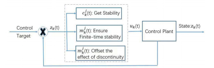
Based on the type-2 Takagi-Sugeno (IT2 T-S) fuzzy theory, a non-autonomous fuzzy complex-valued dynamical system with discontinuous interconnection function is formulated. Under the framework of Filippov, the finite-time stabilization (FTS) problem is investigated by using an indefinite-derivative Lyapunov function method, where the derivative of the constructed Lyapunov function is allowed to be positive. By designing a fuzzy switching state feedback controller involving time-varying control gain parameters, several sufficient criteria are established to determine the considered system's stability in finite time. Correspondingly, due to the time-varying system parameters and the designed time-dependent control gain coefficients, a more flexible settling time (ST) is estimated. Finally, an example is presented to confirm the proposed methodology.
Citation: Xiong Jian, Zengyun Wang, Aitong Xin, Yujing Chen, Shujuan Xie. An improved finite-time stabilization of discontinuous non-autonomous IT2 T-S fuzzy interconnected complex-valued systems: A fuzzy switching state-feedback control method[J]. Electronic Research Archive, 2023, 31(1): 273-298. doi: 10.3934/era.2023014
Based on the type-2 Takagi-Sugeno (IT2 T-S) fuzzy theory, a non-autonomous fuzzy complex-valued dynamical system with discontinuous interconnection function is formulated. Under the framework of Filippov, the finite-time stabilization (FTS) problem is investigated by using an indefinite-derivative Lyapunov function method, where the derivative of the constructed Lyapunov function is allowed to be positive. By designing a fuzzy switching state feedback controller involving time-varying control gain parameters, several sufficient criteria are established to determine the considered system's stability in finite time. Correspondingly, due to the time-varying system parameters and the designed time-dependent control gain coefficients, a more flexible settling time (ST) is estimated. Finally, an example is presented to confirm the proposed methodology.

| [1] |
G. Tanaka, K. Aihara, Complex-valued multistate associative memory with nonlinear multilevel functions for gray-level image reconstruction, IEEE Trans. Neural Networks, 20 (2009), 1463–1473. https://doi.org/10.1109/TNN.2009.2025500 doi: 10.1109/TNN.2009.2025500

|
| [2] | K. Subramanian, R. Savitha, S. Suresh, Complex-valued neuro-fuzzy inference system for wind prediction, in The 2012 International Joint Conference on Neural Networks, IEEE, Brisbane, Australia, (2012), 1–7. https://doi.org/10.1109/IJCNN.2012.6252812 |
| [3] |
R. Song, W. Xiao, H. Zhang, C. Sun, Adaptive dynamic programming for a class of complex-valued nonlinear systems, IEEE Trans. Neural Networks Learn. Syst., 25 (2014), 1733–1739. https://doi.org/10.1109/IJCNN.2012.6252812 doi: 10.1109/IJCNN.2012.6252812
|
| [4] | A. Hirose, Complex-Valued Neural Networks, 2nd edition, Springer-Verlag, New York, 2012. https://doi.org/10.1007/978-3-642-27632-3 |
| [5] |
Z. Wang, X. Liu, Exponential stability of impulsive complex-valued neural networks with time delay, Math. Comput. Simul., 156 (2019), 143–157. https://doi.org/10.1016/j.matcom.2018.07.006 doi: 10.1016/j.matcom.2018.07.006
|
| [6] |
Y. Yu, Z. Zhang, State estimation for complex-valued inertial neural networks with multiple time delays, Mathematics, 10 (2022), 1725. https://doi.org/10.3390/math10101725 doi: 10.3390/math10101725
|
| [7] |
Y. Yu, Z. Zhang, M. Zhong, Z. Wang, Pinning synchronization and adaptive synchronization of complex-valued inertial neural networks with time-varying delays in fixed-time interval, J. Franklin Inst., 359 (2022), 1434–1456 https://doi.org/10.1016/j.jfranklin.2021.11.036 doi: 10.1016/j.jfranklin.2021.11.036
|
| [8] |
M. Ceylan, R. Ceylan, Y. Özbay, S. Kara, Application of complex discrete wavelet transform in classification of Doppler signals using complex-valued artificial neural network, Artif. Intell. Med., 44 (2008), 65–76. https://doi.org/10.1016/j.artmed.2008.05.003 doi: 10.1016/j.artmed.2008.05.003
|
| [9] |
M. E. Valle, Complex-valued recurrent correlation neural networks, IEEE Trans. Neural Networks Learn. Syst., 25 (2014), 1600–1612. https://doi.org/10.1109/TNNLS.2014.2341013 doi: 10.1109/TNNLS.2014.2341013
|
| [10] |
Z. Wang, J. Cao, Z. Guo, L. Huang, Generalized stability for discontinuous complex-valued Hopfield neural networks via differential inclusions, Proc. R. Soc. A, 474 (2018), 20180507. https://doi.org/10.1098/rspa.2018.0507 doi: 10.1098/rspa.2018.0507
|
| [11] |
L. Duan, M. Shi, C. Huang, X. Fang, Synchronization infinite/fixed-time of delayed diffusive complex-valued neural networks with discontinuous activations, Chaos, Solitons Fractals, 142 (2021), 110386. https://doi.org/10.1016/j.chaos.2020.110386 doi: 10.1016/j.chaos.2020.110386
|
| [12] |
Z. Ding, H. Zhang, Z. Zeng, L. Yang, S. Li, Global dissipativity and Quasi-Mittag-Leffler synchronization of fractional-order discontinuous complex-valued neural networks, IEEE Trans. Neural Networks Learn. Syst., 2021 (2021), 1–14. https://doi.org/10.1109/TNNLS.2021.3119647 doi: 10.1109/TNNLS.2021.3119647
|
| [13] | A. Osman, R. Tetzlaff, Modelling brain electrical activity by reaction diffusion cellular nonlinear networks (RD-CNN) in laplace domain, in 2014 14th International Workshop on Cellular Nanoscale Networks and their Applications, IEEE, Notre Dame, USA, (2014), 1–2. https://doi.org/10.1109/CNNA.2014.6888661 |
| [14] |
F. Liu, Y. Li, Y. Cao, J. She, M. Wu, A two-layer active disturbance rejection controller design for load frequency control of interconnected power system, IEEE Trans. Power Syst., 31 (2016), 3320–3321. https://doi.org/10.1109/TPWRS.2015.2480005 doi: 10.1109/TPWRS.2015.2480005
|
| [15] |
L. Su, D. Ye, A cooperative detection and compensation mechanism against Denial-of-Service attack for cyber-physical systems, Inf. Sci., 444 (2018), 122–134. https://doi.org/10.1016/j.ins.2018.02.066 doi: 10.1016/j.ins.2018.02.066
|
| [16] |
H. Wang, W. Liu, J. Qiu, P. X. Liu, Adaptive fuzzy decentralized control for a class of strong interconnected nonlinear systems with unmodeled dynamics, IEEE Trans. Fuzzy Syst., 26 (2018), 836–846. https://doi.org/10.1109/TFUZZ.2017.2694799 doi: 10.1109/TFUZZ.2017.2694799
|
| [17] |
B. Zhao, D. Wang, G. Shi, D. Liu, Y. Li, Decentralized control for large-scale nonlinear systems with unknown mismatched interconnections via policy iteration, IEEE Trans. Syst. Man Cybern. Syst., 48 (2018), 1725–1735. https://doi.org/10.1109/TSMC.2017.2690665 doi: 10.1109/TSMC.2017.2690665
|
| [18] |
P. Bhowmick, A. Dey, Negative imaginary stability result allowing purely imaginary poles in both the interconnected systems, IEEE Control Syst. Lett., 6 (2021), 403–408. https://doi.org/10.1109/LCSYS.2021.3077862 doi: 10.1109/LCSYS.2021.3077862
|
| [19] |
B. Liang, S. Zheng, C. K. Ahn, F. Liu, Adaptive fuzzy control for fractional-order interconnected systems with unknown control directions, IEEE Trans. Fuzzy Syst., 30 (2020), 75–87. https://doi.org/10.1109/TFUZZ.2020.3031694 doi: 10.1109/TFUZZ.2020.3031694
|
| [20] |
P. Gowgi, S. S. Garani, Temporal self-Organization: a reaction-diffusion framework for spatiotemporal memories, IEEE Trans. Neural Networks Learn. Syst., 30 (2018), 427–448. https://doi.org/10.1109/TNNLS.2018.2844248 doi: 10.1109/TNNLS.2018.2844248
|
| [21] |
M. Forti, P. Nistri, Global convergence of neural networks with discontinuous neuron activations, IEEE Trans. Circuits Syst. I Fundam. Theory Appl., 50 (2003), 1421–1435. https://doi.org/10.1109/TCSI.2003.818614 doi: 10.1109/TCSI.2003.818614
|
| [22] |
N. Rong, Z. Wang, H. Zhang, Finite-time stabilization for discontinuous interconnected delayed systems via interval type-2 T-S fuzzy model approach, IEEE Trans. Fuzzy Syst., 27 (2018), 249–261. https://doi.org/10.1109/TFUZZ.2018.2856181 doi: 10.1109/TFUZZ.2018.2856181
|
| [23] |
Z. Wang, N. Rong, H. Zhang, Finite-time decentralized control of IT2 T-S fuzzy interconnected systems with discontinuous interconnections, IEEE Trans. Cybern., 49 (2018), 3547–3556. https://doi.org/10.1109/TCYB.2018.2848626 doi: 10.1109/TCYB.2018.2848626
|
| [24] |
Z. Cai, L. Huang, Z. Wang, X. Pan, L. Zhang, Fixed-time stabilization of IT2 T-S fuzzy control systems with discontinuous interconnections: Indefinite derivative Lyapunov method, J. Franklin Inst., 359 (2022), 2564–2592. https://doi.org/10.1016/j.jfranklin.2022.02.002 doi: 10.1016/j.jfranklin.2022.02.002
|
| [25] |
B. Chen, X. Liu, C. Lin, Observer and adaptive fuzzy control design for nonlinear strict-feedback systems with unknown virtual control coefficients, IEEE Trans. Fuzzy Syst., 26 (2017) 1732–1743. https://doi.org/10.1109/TFUZZ.2017.2750619 doi: 10.1109/TFUZZ.2017.2750619
|
| [26] |
H. Wang, P. X. Liu, X. Zhao, X. Liu, Adaptive fuzzy finite-time control of nonlinear systems with actuator faults, IEEE Trans. Cybern., 50 (2019), 1786–1797. https://doi.org/10.1109/TCYB.2019.2902868 doi: 10.1109/TCYB.2019.2902868
|
| [27] |
T. Takagi, M. Sugeno, Fuzzy identification of systems and its applications to modeling and control, IEEE Trans. Syst. Man Cybern., SMC-15 (1985), 116–132. https://doi.org/10.1109/TSMC.1985.6313399 doi: 10.1109/TSMC.1985.6313399
|
| [28] |
J. M. Mendel, Type-2 fuzzy sets and systems: an overview [corrected reprint], IEEE Comput. Intell. Mag., 2 (2007), 20–29. https://doi.org/10.1109/MCI.2007.380672 doi: 10.1109/MCI.2007.380672
|
| [29] |
Z. Zhu, Y. Pan, Q. Zhou, C. Lu, Event-triggered adaptive fuzzy control for stochastic nonlinear systems with unmeasured states and unknown backlash-like hysteresis, IEEE Trans. Fuzzy Syst., 29 (2020), 1273–1283. https://doi.org/10.1109/TFUZZ.2020.2973950 doi: 10.1109/TFUZZ.2020.2973950
|
| [30] |
S. Tong, X. Min, Y. Li, Observer-based adaptive fuzzy tracking control for strict-feedback nonlinear systems with unknown control gain functions, IEEE Trans. Cybern., 50 (2020), 3903–3913. https://doi.org/10.1109/TCYB.2020.2977175 doi: 10.1109/TCYB.2020.2977175
|
| [31] |
T. Jia, Y. Pan, H. Liang, H. K. Lam, Event-based adaptive fixed-time fuzzy control for active vehicle suspension systems with time-varying displacement constraint, IEEE Trans. Fuzzy Syst., 30 (2021), 2813–2821 https://doi.org/10.1109/TFUZZ.2021.3075490. doi: 10.1109/TFUZZ.2021.3075490
|
| [32] |
B. Xiao, H. K. Lam, Z. Zhong, S. Wen, Membership-Function-Dependent stabilization of event-triggered interval Type-2 polynomial fuzzy-model-based networked control systems, IEEE Trans. Fuzzy Syst., 28 (2019), 3171–3180. https://doi.org/10.1109/TFUZZ.2019.2957256 doi: 10.1109/TFUZZ.2019.2957256
|
| [33] |
X. Li, T. Huang, J. A. Fang, Event-triggered stabilization for Takagi-Sugeno fuzzy complex-valued Memristive neural networks with mixed time-varying delay, IEEE Trans. Fuzzy. Syst., 29 (2020), 1853–1863. https://doi.org/10.1109/TFUZZ.2020.2986713 doi: 10.1109/TFUZZ.2020.2986713
|
| [34] |
J. Jian, P. Wan, Global exponential convergence of fuzzy complex-valued neural networks with time-varying delays and impulsive effects, Fuzzy Sets Syst., 338 (2018), 23–39. https://doi.org/10.1016/j.fss.2017.12.001 doi: 10.1016/j.fss.2017.12.001
|
| [35] |
S. P. Bhat, D. S. Bernstein, Finite-time stability of continuous autonomous systems, SIAM J. Control Optim., 38 (2000), 751–766. https://doi.org/10.1137/S0363012997321358 doi: 10.1137/S0363012997321358
|
| [36] |
E. Moulay, W. Perruquetti, Finite time stability of differential inclusions, IMA J. Math. Control Inf., 22 (2005), 465–475. https://doi.org/10.1093/imamci/dni039 doi: 10.1093/imamci/dni039
|
| [37] |
Z. Wang, J. Cao, Z. Cai, Sufficient conditions on finite-time input-to-state stability of nonlinear impulsive systems: a relaxed Lyapunov function method, Int. J. Control, 2021 (2021), 1–10. https://doi.org/10.1080/00207179.2021.1949044 doi: 10.1080/00207179.2021.1949044
|
| [38] |
L. Hua, H. Zhu, S. Zhong, Y. Zhang, K. Shi, O. M. Kwon, Fixed-time stability of nonlinear impulsive systems and its Application to inertial neural networks, IEEE Trans. Neural Networks Learn. Syst., 2022 (2022), 1–12. https://doi.org/10.1109/TNNLS.2022.3185664 doi: 10.1109/TNNLS.2022.3185664
|
| [39] | A. Filippov, Differential equations with discontinuous right-hand sides, Springer Dordrecht, 1988. http://dx.doi.org/10.1007/978-94-015-7793-9 |
| [40] |
Z. Wang, J. Cao, Z. Cai, M. Abdel-Aty, A novel Lyapunov theorem on finite/fixed-time stability of discontinuous impulsive systems, Chaos, 30 (2020), 013139. https://doi.org/10.1063/1.5121246 doi: 10.1063/1.5121246
|
| [41] | G. H. Hardy, J. E. Littlewood, G. Polya, Inequalities, Cambridge university press, 1988. https://www.cambridge.org/9780521358804 |
| [42] |
Z. Zhong, Y. Zhu, H. K. Lam, Asynchronous piecewise output-feedback control for large-scale fuzzy systems via distributed event-triggering schemes, IEEE Trans. Fuzzy Syst., 26 (2017), 1688–1703. https://doi.org/10.1109/TFUZZ.2017.2744599 doi: 10.1109/TFUZZ.2017.2744599
|
| [43] |
Z. Wu, G. Chen, X. Fu, Synchronization of a network coupled with complex-variable chaotic systems, Chaos, 22 (2012), 023127. https://doi.org/10.1063/1.4717525 doi: 10.1063/1.4717525
|
| [44] |
B. Chen, X. Liu, S. Tong, Adaptive fuzzy approach to control unified chaotic systems, Chaos, Solitons Fractals, 34 (2007), 1180–1187. https://doi.org/10.1016/j.chaos.2006.04.035 doi: 10.1016/j.chaos.2006.04.035
|


Figures(19) / Tables(2)
Xiong Jian, Zengyun Wang, Aitong Xin, Yujing Chen, Shujuan Xie. An improved finite-time stabilization of discontinuous non-autonomous IT2 T-S fuzzy interconnected complex-valued systems: A fuzzy switching state-feedback control method[J]. Electronic Research Archive, 2023, 31(1): 273-298. doi: 10.3934/era.2023014


 DownLoad: