Pulse diagnosis, also known as Nadi Pariksha, is one of the various diagnostic modalities used in Ayurveda. Nadi Pariksha is a way of determining the underlying cause of a sickness that needs extensive knowledge of the Tridosha signals (i.e. Vata, Pitta and Kapha), as well as the peculiarities of each pulse signal and their relationship to each dominant signal. A Nadi expert can gain a sense of the patient's health status by using this approach and then provide treatment based on that information. In the present day, the health monitoring of people has become an essential requirement. A system which keeps track of the patient's health and continuously captures pulse signals will be helpful. In this work a healthcare monitoring system that uses sensors was developed, and the analysis of Vata, Pitta and Kapha for various patients is discussed, as well as the uploading of the same data to a self-made IoT cloud. The mean values of Vata, Pita and Kapha were compared for different age groups; we found that it is more significant for the age group of 41‒50.
Citation: Sanjay Dubey, M. C. Chinnaiah, I. A. Pasha, K. Sai Prasanna, V. Praveen Kumar, R. Abhilash. An IoT based Ayurvedic approach for real time healthcare monitoring[J]. AIMS Electronics and Electrical Engineering, 2022, 6(3): 329-344. doi: 10.3934/electreng.2022020
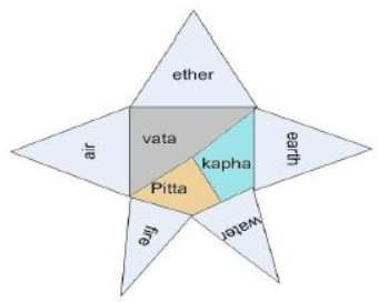
Pulse diagnosis, also known as Nadi Pariksha, is one of the various diagnostic modalities used in Ayurveda. Nadi Pariksha is a way of determining the underlying cause of a sickness that needs extensive knowledge of the Tridosha signals (i.e. Vata, Pitta and Kapha), as well as the peculiarities of each pulse signal and their relationship to each dominant signal. A Nadi expert can gain a sense of the patient's health status by using this approach and then provide treatment based on that information. In the present day, the health monitoring of people has become an essential requirement. A system which keeps track of the patient's health and continuously captures pulse signals will be helpful. In this work a healthcare monitoring system that uses sensors was developed, and the analysis of Vata, Pitta and Kapha for various patients is discussed, as well as the uploading of the same data to a self-made IoT cloud. The mean values of Vata, Pita and Kapha were compared for different age groups; we found that it is more significant for the age group of 41‒50.

| [1] |
Kurande V, Waagepetersen R, Toft E, et al. (2012) Repeatability of Pulse Diagnosis and Body Constitution Diagnosis in Traditional Indian Ayurveda Medicine. Global advances in health and medicine 1: 36–42. https://doi.org/10.7453/gahmj.2012.1.5.011 doi: 10.7453/gahmj.2012.1.5.011

|
| [2] |
Roopini N, Shivaram JM, Shridhar D (2015) Design & Development of a System for Nadi Pariksha. International Journal of Engineering Research Technology (IJERT) 4: 465‒470. http://dx.doi.org/10.17577/IJERTV4IS060509 doi: 10.15623/ijret.2015.0406080
|
| [3] | Narayanan C, Kumar AD, Priyadharshini S, et al. (2015) Cardiac Disorder Diagnosis through Nadi (Pulse) using Piezo Electric Sensors. International Journal of Multidisciplinary Research and Modern Education (IJMRME) 1: 209‒214. |
| [4] | Lad V (2007) Secrets of the Pulse: The ancient art of Ayurvedic pulse diagnosis. 2 Eds., Delhi: Motilal Banarsidass Publishing House. |
| [5] |
Navghare S, Bajaj P (2018) Design of Non-Invasive Pulse Rate Detector using LabVIEW. International Journal of Computer Applications 181: 19‒24. http://dx.doi.org/10.5120/ijca2018917811 doi: 10.5120/ijca2018917811
|
| [6] |
Anu S, Devi R, Keerthana R, et al. (2015) PC based Monitoring of Human Pulse Signal using LabVIEW. International Journal of Innovative Research in Electrical, Electronics, Instrumentation and Control Engineering 3: 186‒187. http://dx.doi.org/10.17148/IJIREEICE.2015.3344 doi: 10.17148/IJIREEICE.2015.3344
|
| [7] |
Kalange AE, Gangal SA (2007) Piezoelectric Sensor for Human Pulse Detection. Defence Sci J 57: 109‒114. https://doi.org/10.14429/dsj.57.1737 doi: 10.14429/dsj.57.1737
|
| [8] |
Pavana MG, Shashikala N, Joshi M (2016) Design, development and comparative performance analysis of Bessel and Butterworth filter for Nadi Pariksha Yantra. 2016 IEEE International Conference on Engineering and Technology (ICETECH), 1068‒1072. https://doi.org/10.1109/ICETECH.2016.7569413 doi: 10.1109/ICETECH.2016.7569413
|
| [9] |
Kalange AE, Mahale BP, Aghav ST, et al. (2012) Nadi Parikshan Yantra and analysis of radial pulse. 1st International Symposium on Physics and Technology of Sensors (ISPTS-1), 165‒168. https://doi.org/10.1109/ISPTS.2012.6260910 doi: 10.1109/ISPTS.2012.6260910
|
| [10] |
Yoon YZ, Lee MH, Soh KS (2000) Pulse type classification by varying contact pressure. IEEE Eng Med Biol 19: 106‒110. https://doi.org/10.1109/51.887253 doi: 10.1109/51.887253
|
| [11] |
Sorvoja H, Kokko VM, Myllyla R, et al. (2005) Use of EMFi as a blood pressure pulse transducer. IEEE Transactions on Instrumentation and Measurement 54: 2505‒2512. https://doi.org/10.1109/TIM.2005.853345 doi: 10.1109/TIM.2005.853345
|
| [12] |
Chaudhari S, Mudhalwadkar R (2017) Nadi pariksha system for health diagnosis. International Conference on Intelligent Computing and Control (I2C2), 1‒4. https://doi.org/10.1109/I2C2.2017.8321935 doi: 10.1109/I2C2.2017.8321935
|
| [13] |
Škraba A, Koložvari A, Kofjač D, et al. (2019) Prototype of Group Heart Rate Monitoring with ESP32. 8th Mediterranean Conference on Embedded Computing (MECO), 1‒4. https://doi.org/10.1109/MECO.2019.8760150 doi: 10.1109/MECO.2019.8760150
|
| [14] |
Khaire NN, Joshi YV (2015) Diagnosis of Disease Using Wrist Pulse Signal for classification of pre-meal and post-meal samples. International Conference on Industrial Instrumentation and Control (ICIC), 866‒869. https://doi.org/10.1109/IIC.2015.7150864 doi: 10.1109/IIC.2015.7150864
|
| [15] |
Khandai SK, Jain SK (2017) Comparison of sensors performance for the development of wrist pulse acquisition system. TENCON 2017 IEEE Region 10 Conference, 2870‒2875. https://doi.org/10.1109/TENCON.2017.8228351. doi: 10.1109/TENCON.2017.8228351
|
| [16] |
Lee J, Kim J, Lee M (2001) Design of Digital Hardware System for Pulse Signals. J Med Syst 25: 385–394. https://doi.org/10.1023/A:1011975727571 doi: 10.1023/A:1011975727571
|
| [17] | Krishnan S, Abudhahir A (2016) Development of system to acquire Radial Artery Pulse for Objective Pain Measurement. Biomedicine 36: 35‒40. |
| [18] |
Joshi A, Kulkarni A, Chandran S, et al. (2007) Nadi Tarangini: A Pulse Based Diagnostic System. 29th Annual International Conference of the IEEE Engineering in Medicine and Biology Society, 2207‒2210. https://doi.org/10.1109/IEMBS.2007.4352762 doi: 10.1109/IEMBS.2007.4352762
|
| [19] |
Pereira T, Paiva JS, Correia C, et al. (2016) An automatic method for arterial pulse waveform recognition using KNN and SVM classifiers. Med Biol Eng Comput 54: 1049–1059. https://doi.org/10.1007/s11517-015-1393-5 doi: 10.1007/s11517-015-1393-5
|
| [20] |
Rao S, Rao R (2015) Investigation on pulse reading using flexible pressure sensor. International Conference on Industrial Instrumentation and Control (ICIC), 213‒216. https://doi.org/10.1109/IIC.2015.7150740 doi: 10.1109/IIC.2015.7150740
|
| [21] |
Valsalan P, Baomar TA, Baabood AH (2020) IOT Based Health Monitoring System. Journal of Critical Reviews 7: 739‒743. https://doi.org/10.31838/jcr.07.04.137 doi: 10.31838/jcr.07.04.137
|
| [22] | Murphy J, Gitman Y, Pulse Sensor. Open Hardware. Available from: https://pulsesensor.com/pages/open-hardware |
| [23] |
Sareen M, Kumar M, Santhosh J, et al. (2009) Nadi Yantra: a robust system design to capture the signals from the radial artery for assessment of the autonomic nervous system non-invasively. Journal of Biomedical Science and Engineering 2: 471‒479. https://doi.org/10.4236/jbise.2009.27068 doi: 10.4236/jbise.2009.27068
|
| [24] | Thakker B, Vyas AL (2009) Outlier Pulse Detection and Feature Extraction for Wrist Pulse Analysis. International Journal of Biomedical and Biological Engineering 3: 127‒130. |
| [25] | Highlights of Nadi Tarangini. Available from: https://www.naditarangini.com/nadi-tarangini-device/ |
| [26] |
Das S, Namasudra S (2022) A novel hybrid encryption method to secure healthcare data in IoT-enabled healthcare infrastructure. Comput Electr Eng 101: 107991. https://doi.org/10.1016/j.compeleceng.2022.107991 doi: 10.1016/j.compeleceng.2022.107991
|
| [27] |
Gupta A, Namasudra S (2022) A novel technique for accelerating live migration in cloud computing, Automat Softw Eng 29: 1‒21. https://doi.org/10.1007/s10515-022-00332-2 doi: 10.1007/s10515-021-00310-0
|
| [28] |
Das S, Namasudra S (2022) MACPABE: Multi authority-based CP-ABE with efficient attribute revocation for IoT-enabled healthcare infrastructure. Int J Netw Manag, e2200. https://doi.org/10.1002/nem.2200 doi: 10.1002/nem.2200
|
| [29] |
Kumar A, Abhishek K, Namasudra S, et al. (2021) A novel elliptic curve cryptography based system for smart grid communication. Int J Web Grid Serv 17: 321‒342. https://doi.org/10.1504/IJWGS.2021.10040914 doi: 10.1504/IJWGS.2021.118398
|
| [30] | Bawankar BU, Dharmik RC, Telrandhe S (2021) Nadi pariksha: IOT-based patient monitoring and disease prediction system. InJournal of Physics: Conference Series 1913: 012124. IOP Publishing. https://doi.org/10.1088/1742-6596/1913/1/012124 |
| [31] | Kashyap M, Jain S (2022) Importance of Pulse Examination and Its Diagnostic System. In Recent Innovations in Computing, 189‒199. Springer, Singapore. https://doi.org/10.1007/978-981-16-8248-3_16 |


Figures(13) / Tables(1)

Sanjay Dubey, M. C. Chinnaiah, I. A. Pasha, K. Sai Prasanna, V. Praveen Kumar, R. Abhilash. An IoT based Ayurvedic approach for real time healthcare monitoring[J]. AIMS Electronics and Electrical Engineering, 2022, 6(3): 329-344. doi: 10.3934/electreng.2022020


 DownLoad: