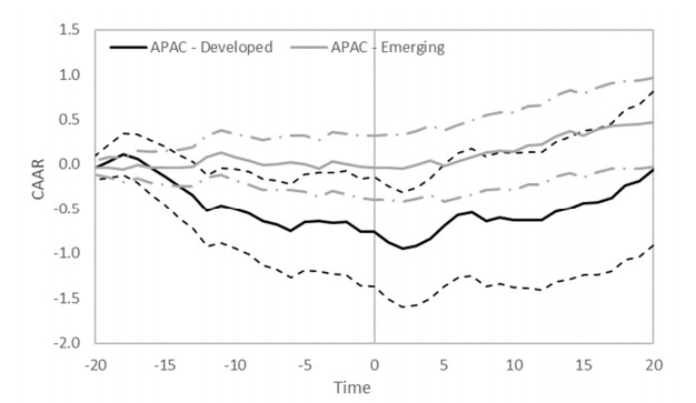
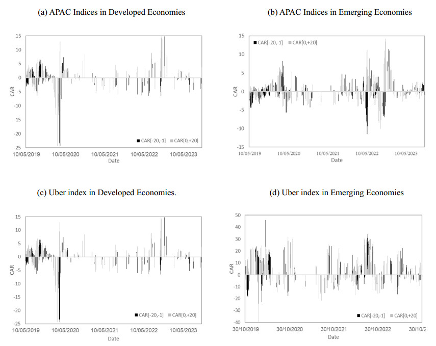
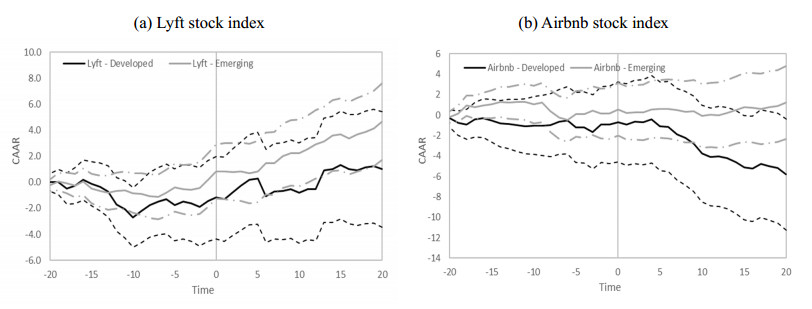
I investigated Uber's strategic announcements' impact on stock markets within the Asia Pacific region, distinguishing developed and emerging economies. Utilizing Crunchbase.com data, I applied the "Index Impact Test" and "Stock Response Test" to analyze market responses. I found that in developed economies, stock indices experienced a negative trend before announcements and a positive trend thereafter. In contrast, emerging economies exhibited a positive response exclusively after announcements. I also explored the performance of Uber's stock, demonstrating positive post-announcement effects in both economy types, with emerging economies showing sustained positivity. Further, I expanded to assess Uber's influence on other peer-to-peer (P2P) companies, specifically Lyft and Airbnb, offering insights into the broader implications of Uber's announcements across the P2P sector. The findings suggested that Lyft received a positive market response in developed and emerging economies, while Airbnb's response in developed economies tended to be negative post-announcement.
Citation: Tchai Tavor. Exploring the heterogeneity of stock market responses to Uber announcements: A comparative analysis of developed and emerging economies in Asia Pacific[J]. Quantitative Finance and Economics, 2024, 8(2): 315-346. doi: 10.3934/QFE.2024012
I investigated Uber's strategic announcements' impact on stock markets within the Asia Pacific region, distinguishing developed and emerging economies. Utilizing Crunchbase.com data, I applied the "Index Impact Test" and "Stock Response Test" to analyze market responses. I found that in developed economies, stock indices experienced a negative trend before announcements and a positive trend thereafter. In contrast, emerging economies exhibited a positive response exclusively after announcements. I also explored the performance of Uber's stock, demonstrating positive post-announcement effects in both economy types, with emerging economies showing sustained positivity. Further, I expanded to assess Uber's influence on other peer-to-peer (P2P) companies, specifically Lyft and Airbnb, offering insights into the broader implications of Uber's announcements across the P2P sector. The findings suggested that Lyft received a positive market response in developed and emerging economies, while Airbnb's response in developed economies tended to be negative post-announcement.

| [1] |
Alvarez F, Argente D (2022) On the effects of the availability of means of payments: The case of uber. Q J Econ 137: 1737–1789. https://doi.org/10.1093/qje/qjac008 doi: 10.1093/qje/qjac008

|
| [2] |
Ball R, Brown P (1968) An empirical evaluation of accounting income numbers. J Account Res 6: 159–178. https://doi.org/10.2307/2490232 doi: 10.2307/2490232
|
| [3] | Barreto Y, Neto RDMS, Carazza L (2021) Uber and traffic safety: Evidence from Brazilian cities. J Urban Econ 123: 103347. https://doi.org/10.1016/j.jue.2021.103347 |
| [4] |
Basu A (2019) Viability assessment of emerging smart urban para-transit solutions: Case of cab aggregators in Kolkata city, India. J Urban Manage 8: 364–376. https://doi.org/10.1016/j.jum.2019.01.002 doi: 10.1016/j.jum.2019.01.002
|
| [5] |
Bianco S, Zach FJ, Singal M (2022b) Disruptor recognition and market value of incumbent firms: Airbnb and the lodging industry. J Hosp Tour Res 48: 84–104. https://doi.org/10.1177/10963480221085215 doi: 10.1177/10963480221085215
|
| [6] | Borio C (2014) The financial cycle and macroeconomics: What have we learnt? J Bank Financ 45: 182–198. https://doi.org/10.1016/j.jbankfin.2013.07.031 |
| [7] |
Brown SJ, Warner JB (1985) Using daily stock returns: The Case of Event Studies. J Financ Econ 14: 3-31. https://doi.org/10.1016/0304-405X(85)90042-X doi: 10.1016/0304-405X(85)90042-X
|
| [8] |
Celik MS, Ozturk MB, Haykir O (2024) The effect of technological developments on the stock market: evidence from emerging market. Appl Econ Lett 31: 118–121. https://doi.org/10.1080/13504851.2022.2128172 doi: 10.1080/13504851.2022.2128172
|
| [9] |
Choi TM, He Y (2019) Peer-to-peer collaborative consumption for fashion products in the sharing economy: Platform operations. Transport Res Part E 126: 49–65. https://doi.org/10.1016/j.tre.2019.03.016 doi: 10.1016/j.tre.2019.03.016
|
| [10] |
Cohen B, Kietzmann J (2014) Ride on! Mobility business models for the sharing economy. Organ Environ 27: 279–296. https://doi.org/10.1177/1086026614546199 doi: 10.1177/1086026614546199
|
| [11] |
Comin D, Nanda R (2019) Financial development and technology diffusion. IMF Econ Rev 67: 395–419. https://doi.org/10.1057/s41308-019-00078-0 doi: 10.1057/s41308-019-00078-0
|
| [12] | Conway MW, Salon D, King DA (2018) Trends in taxi use and the advent of ridehailing, 1995–2017: Evidence from the US National Household Travel Survey. Urban Sci 2: 79. https://doi.org/10.3390/urbansci2030079 |
| [13] |
Cowan AR (1992) Nonparametric event study tests. Rev Quant Financ Account 2: 343–358. https://doi.org/10.1007/BF00939016 doi: 10.1007/BF00939016
|
| [14] |
Cramer J, Krueger AB (2016) Disruptive change in the taxi business: The case of Uber. Am Econ Rev 106: 177–182. https://doi.org/10.1257/aer.p20161002 doi: 10.1257/aer.p20161002
|
| [15] |
Deller S, Watson P (2016) Spatial variations in the relationship between economic diversity and stability. Appl Econ Lett 23: 520–525. https://doi.org/10.1080/13504851.2015.1085630 doi: 10.1080/13504851.2015.1085630
|
| [16] |
Dolnicar S (2021) Sharing economy and peer-to-peer accommodation–a perspective paper. Tour Rev 76: 34–37. https://doi.org/10.1108/TR-05-2019-0197 doi: 10.1108/TR-05-2019-0197
|
| [17] |
Doner RF, Hicken A, Ritchie BK (2009) Political Challenges of Innovation in the Developing World 1. Rev Policy Res 26: 151–171. https://doi.org/10.1111/j.1541-1338.2008.00373.x doi: 10.1111/j.1541-1338.2008.00373.x
|
| [18] | Edelman BG, Geradin D (2015) Efficiencies and regulatory shortcuts: How should we regulate companies like Airbnb and Uber. Stan Tech L Rev 19: 293. https://doi.org/10.2139/ssrn.2658603 |
| [19] |
Fama EF (1970) Efficient capital markets: A review of theory and empirical work. J Financ 25: 383–417. https://doi.org/10.1111/j.1540-6261.1970.tb00518.x doi: 10.1111/j.1540-6261.1970.tb00518.x
|
| [20] | Fama EF, Fisher L, Jensen MC, et al. (1969) The adjustment of stock prices to new information. Int Econ Rev 10: 1–21. https://www.jstor.org/stable/2525569 |
| [21] | Gagnon JE, Kamin SB, Kearns J (2023) The impact of the COVID-19 pandemic on global GDP growth. J JPN Int Econ 68: 101258. https://doi.org/10.1016/j.jjie.2023.101258 |
| [22] |
Gao M, Yen J, Liu M (2021) Determinants of defaults on P2P lending platforms in China. Int Rev Econ Financ 72: 334–348. https://doi.org/10.1016/j.iref.2020.11.012 doi: 10.1016/j.iref.2020.11.012
|
| [23] |
Gavalas D, Syriopoulos T, Tsatsaronis M (2022) COVID–19 impact on the shipping industry: An event study approach. Transport Policy 116: 157–164. https://doi.org/10.1016/j.tranpol.2021.11.016 doi: 10.1016/j.tranpol.2021.11.016
|
| [24] | Grassini L (2023) Statistical features and economic impact of Covid-19 (Editoriale). National Account Rev 5: 38–40. https://doi:10.3934/NAR.2023003" target="_blank">10.3934/NAR.2023003">https://doi:10.3934/NAR.2023003 |
| [25] |
Hall JV, Krueger AB (2018) An analysis of the labor market for Uber's driver-partners in the United States. ILR Rev 71: 705–732. https://doi.org/10.1177/0019793917717222 doi: 10.1177/0019793917717222
|
| [26] | Hall JD, Palsson C, Price J (2018) Is Uber a substitute or complement for public transit? J Urban Econ 108: 36–50. https://doi.org/10.1016/j.jue.2018.09.003 |
| [27] |
Hasan N, Khan AG, Hossen MA, et al. (2021) Ride on Conveniently!: Passengers' Adoption of Uber App in an Emerging Economy. Int J e-Adoption (IJEA) 13: 19–35. https://doi.org/10.4018/IJEA.2021070102 doi: 10.4018/IJEA.2021070102
|
| [28] | Huang C, Zhang M, Wang C, et al. (2022) An interactive two-stage retail electricity market for microgrids with peer-to-peer flexibility trading. Appl Energy 320: 119085. https://doi.org/10.1016/j.apenergy.2022.119085 |
| [29] |
Junarsin E, Hanafi MM, Iman N, et al. (2023) Can technological innovation spur economic development? The case of Indonesia. J Sci Technol Policy Manage 14: 25–52. https://doi.org/10.1108/JSTPM-12-2020-0169 doi: 10.1108/JSTPM-12-2020-0169
|
| [30] | Kartika R (2023) Financial Technology Innovation-Peer-to-Peer (P2P) Lending in the RCEP Member States, Regional Comprehensive Economic Partnership, 93. https://doi.org/10.2174/9789815123227123010010 |
| [31] |
Katz LF, Krueger AB (2019) The rise and nature of alternative work arrangements in the United States, 1995–2015. ILR Rev 72: 382–416. https://doi.org/10.1177/0019793918820008 doi: 10.1177/0019793918820008
|
| [32] | Ki D, Lee S (2019) Spatial distribution and location characteristics of Airbnb in Seoul, Korea. Sustainability 11: 4108. https://doi.org/10.3390/su11154108 |
| [33] | Kiatkawsin K, Sutherland I, Kim JY (2020) A comparative automated text analysis of Airbnb reviews in Hong Kong and Singapore using latent dirichlet allocation. Sustainability 12: 6673. https://doi.org/10.3390/su12166673 |
| [34] | Kim B (2019) Understanding key antecedents of consumer loyalty toward sharing-economy platforms: The case of Airbnb. Sustainability 11: 5195. https://doi.org/10.3390/su11195195 |
| [35] | Kim HJ, Suh CS (2021) Spreading the sharing economy: Institutional conditions for the international diffusion of Uber, 2010-2017. Plos One 16: e0248038. https://doi.org/10.1371/journal.pone.0248038 |
| [36] |
Kim K, Baek C, Lee JD (2018) Creative destruction of the sharing economy in action: The case of Uber. Transp Res Part A: Policy Pract 110: 118–127. https://doi.org/10.1016/j.tra.2018.01.014 doi: 10.1016/j.tra.2018.01.014
|
| [37] |
Kolari JW, Pynnönen S (2010) Event study testing with cross-sectional correlation of abnormal returns. Rev Financ Stud 23: 3996–4025. https://doi.org/10.1093/rfs/hhq072 doi: 10.1093/rfs/hhq072
|
| [38] |
Koh E, King B (2017) Accommodating the sharing revolution: a qualitative evaluation of the impact of Airbnb on Singapore's budget hotels. Tour Recreat Res 42: 409–421. https://doi.org/10.1080/02508281.2017.1314413 doi: 10.1080/02508281.2017.1314413
|
| [39] |
Kuhzady S, Seyfi S, Béal L (2022) Peer-to-peer (P2P) accommodation in the sharing economy: A review. Current Issues Tour 25: 3115–3130. https://doi.org/10.1080/13683500.2020.1786505 doi: 10.1080/13683500.2020.1786505
|
| [40] |
Kwak J, Chang SY, Jin M (2023) The effects of political ties on innovation performance in China: Differences between central and local governments. Asian Bus Manage 22: 300–329. https://doi.org/10.1057/s41291-021-00167-x doi: 10.1057/s41291-021-00167-x
|
| [41] |
Li T, Zhong J, Huang Z (2019) Potential dependence of financial cycles between emerging and developed countries: Based on ARIMA-GARCH Copula model. Emerg Mark Financ Tr 56: 1237–1250. https://doi.org/10.1080/1540496X.2019.1611559 doi: 10.1080/1540496X.2019.1611559
|
| [42] | Liu W, Xia LQ (2017) An evolutionary behavior forecasting model for online lenders and borrowers in peer-to-peer lending. Asia-Pac J Oper Res 34: 1740008. https://doi.org/10.1142/S0217595917400085 |
| [43] | Lopes M, Teixeira AA (2009) Open Innovation in firms located in an intermediate technology developed country. Inst Syst Comput Eng Porto. |
| [44] | Maneenop S, Kotcharin S (2020) The impacts of COVID-19 on the global airline industry: An event study approach. J Air Transport Management 89: 101920. https://doi.org/10.1016/j.jairtraman.2020.101920 |
| [45] |
McDonald C (2010) Technology in the political landscape. IEEE Ann History Comput 32: 87–88. https://doi:10.1109/MAHC.2010.42 doi: 10.1109/MAHC.2010.42
|
| [46] | MacKinlay AC (1997) Event studies in economics and finance. J Econ Lit 35: 13–39. https://www.jstor.org/stable/2729691 |
| [47] | Munasinghe LM, Gunawardhana T, Wickramaarachchi NC, et al. (2022) Regulation of peer-to-peer tourist accommodation services: lessons from Asia pacific countries for Sri Lanka. Revista Produção e Desenvolvimento 8: e593–e593. https://doi.org/10.32358/rpd.2022.v8.593 |
| [48] |
Oh EY, Rosenkranz P (2022) Determinants of peer-to-peer lending expansion: The roles of financial development and financial literacy. J FinTech, 2250001. https://doi.org/10.1142/S2705109922500018 doi: 10.1142/S2705109922500018
|
| [49] | Palatnik RR, Tavor T, Voldman L (2019) The Symptoms of Illness: Does Israel Suffer from "Dutch Disease"? Energies 12: 2752. https://doi.org/10.3390/en12142752 |
| [50] | Patell JM (1976) Corporate forecasts of earnings per share and stock price behavior: Empirical test. J Account Res, 246–276. https://www.jstor.org/stable/2490543 |
| [51] |
Plouffe CR (2008) Examining "peer-to-peer"(P2P) systems as consumer-to-consumer (C2C) exchange. Eur J Market 42: 1179–1202. https://doi.org/10.1108/03090560810903637 doi: 10.1108/03090560810903637
|
| [52] |
Puche ML (2019) Regulation of TNCs in Latin America: The case of uber regulation in Mexico City and Bogota. The Governance of Smart Transportation Systems: Towards New Organizational Structures for the Development of Shared, Automated, Electric and Integrated Mobility, 37–53. https://doi.org/10.1007/978-3-319-96526-0_3 doi: 10.1007/978-3-319-96526-0_3
|
| [53] | Quattrone G, Kusek N, Capra L (2022) A global-scale analysis of the sharing economy model-an AirBnB case study. EPJ Data Sci 11: 36. https://doi.org/10.1140/epjds/s13688-022-00349-3 |
| [54] | Rahman MH, Sadeek SN, Ahmed A, et al. (2021) Effect of socio-economic and demographic factors on ride-sourcing services in Dhaka City, Bangladesh. Transp Res Interdiscipl Perspect 12: 100492. https://doi.org/10.1016/j.trip.2021.100492 |
| [55] | Rauch DE, Schleicher D (2015) Like Uber, but for local government law: the future of local regulation of the sharing economy. George Mason Law and Economics Research Paper No. 15-01. https://doi.org/10.2139/ssrn.2549919 |
| [56] | Roy A, Bruce A, MacGill I (2016) The potential value of peer-to-peer energy trading in the Australian national electricity market. In Asia-pacific solar research conference. |
| [57] |
Rudny W (2018) Financialization and its impact upon the developed economies. Ekonomiczne Problemy Usług 131: 315–322. https://doi.org/10.18276/epu.2018.131/1-31 doi: 10.18276/epu.2018.131/1-31
|
| [58] | Schneiders A, Fell MJ, Nolden C (2022) Peer-to-peer electricity trading and the sharing economy: social, markets and regulatory perspectives. Energ Source Part B 17: 2050849. https://doi.org/10.1080/15567249.2022.2050849 |
| [59] | Song P, Zhou Y, Yuan J (2021) Peer-to-peer trade and the economy of distributed PV in China. J Clean Prod 280: 124500. https://doi.org/10.1016/j.jclepro.2020.124500 |
| [60] | Stafford TF, Duong BQ (2023) Social media in emerging economies: A cross-cultural comparison. IEEE Transact Comput Social Syst 10: 1160–1178. https://doi:10.1109/TCSS.2022.3169412 |
| [61] | Sundararajan A (2017) The sharing economy: The end of employment and the rise of crowd-based capitalism, MIT press. |
| [62] | Surie A, Koduganti J (2016) The emerging nature of work in platform economy companies in Bengaluru, India: The case of Uber and Ola Cab drivers. E-J Int Compe Labour Stud. |
| [63] |
Tan KPS, Yang Y, Li XR (2022) Catching a ride in the peer-to-peer economy: Tourists' acceptance and use of ridesharing services before and during the COVID-19 pandemic. J Bus Res 151: 504–518. https://doi.org/10.1016/j.jbusres.2022.05.069 doi: 10.1016/j.jbusres.2022.05.069
|
| [64] |
Tavor T (2023) The effect of natural gas discoveries in Israel on the strength of its currency. Aust Econ Pap 62: 236–256. https://doi.org/10.1111/1467-8454.12296 doi: 10.1111/1467-8454.12296
|
| [65] | Tavor T (2024) Impact of announcements on capital market performance in emerging markets: a parametric and non-parametric analysis. Int J Emerg Mark. https://doi.org/10.1108/IJOEM-05-2023-0852 |
| [66] |
Teitler-Regev S, Tavor T (2023) The effect of Airbnb announcements on hotel stock prices. Aus Econ Pap 62: 78–100. https://doi.org/10.1111/1467-8454.12281 doi: 10.1111/1467-8454.12281
|
| [67] | Teitler-Regev S, Tavor T (2024) Analyzing the varied impact of COVID-19 on stock markets: A comparative study of low-and high-infection-rate countries. Plos One 19: e0296673. https://doi.org/10.1371/journal.pone.0296673 |
| [68] | Tumbali MVL (2020) Impact of AirBnB on Philippine accommodation sector: A quantitative approach. J Tour Hosp Environ Manage 5: 74–88. https://doi.org/10/35631/JTHEM.521005 |
| [69] |
Tzur A (2019) Uber Über regulation? Regulatory change following the emergence of new technologies in the taxi market. Regul Govern 13: 340–361. https://doi.org/10.1111/rego.12170 doi: 10.1111/rego.12170
|
| [70] |
Valdez J (2023) The politics of Uber: Infrastructural power in the United States and Europe. Regul Govern 17: 177–194. https://doi.org/10.1111/rego.12456 doi: 10.1111/rego.12456
|
| [71] | Vinogradov E, Leick B, Kivedal BK (2020) An agent-based modelling approach to housing market regulations and Airbnb-induced tourism. Tour Manage 77: 104004. https://doi.org/10.1016/j.tourman.2019.104004 |
| [72] | Vollans GE (2004) Restructuring the regulatory framework in developing countries. Ener Stud Rev 12. https://doi.org/10.15173/esr.v12i2.457 |
| [73] |
Wang Z (2023) The Impact of COVID-19 on Economic Development. Highlights Bus Econ Manage 14: 257–262. https://doi.org/10.54097/hbem.v14i.9200 doi: 10.54097/hbem.v14i.9200
|
| [74] | Wilcoxon F (1945) Individual comparisons by ranking methods, Breakthroughs in Statistics, 196–202. https://doi.org/10.1007/978-1-4612-4380-9_16 |
| [75] | Zhang M, Geng R, Huang Y, et al. (2021) Terminator or accelerator? Lessons from the peer-to-peer accommodation hosts in China in responses to COVID-19. Int J Hosp Manage 92: 102760. https://doi.org/10.1016/j.ijhm.2020.102760 |
| [76] |
Zhao L, Rasoulinezhad E, Sarker T, et al. (2023) Effects of COVID-19 on global financial markets: evidence from qualitative research for developed and developing economies. Eur J Dev Res 35: 148–166. https://doi.org/10.1057/s41287-021-00494-x doi: 10.1057/s41287-021-00494-x
|

Figures(4) / Tables(6)

Tchai Tavor. Exploring the heterogeneity of stock market responses to Uber announcements: A comparative analysis of developed and emerging economies in Asia Pacific[J]. Quantitative Finance and Economics, 2024, 8(2): 315-346. doi: 10.3934/QFE.2024012


 DownLoad: