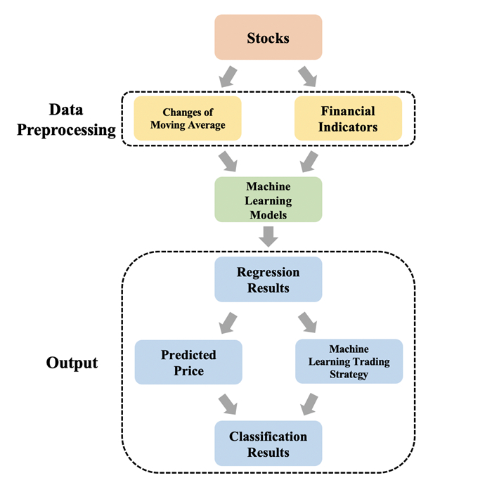
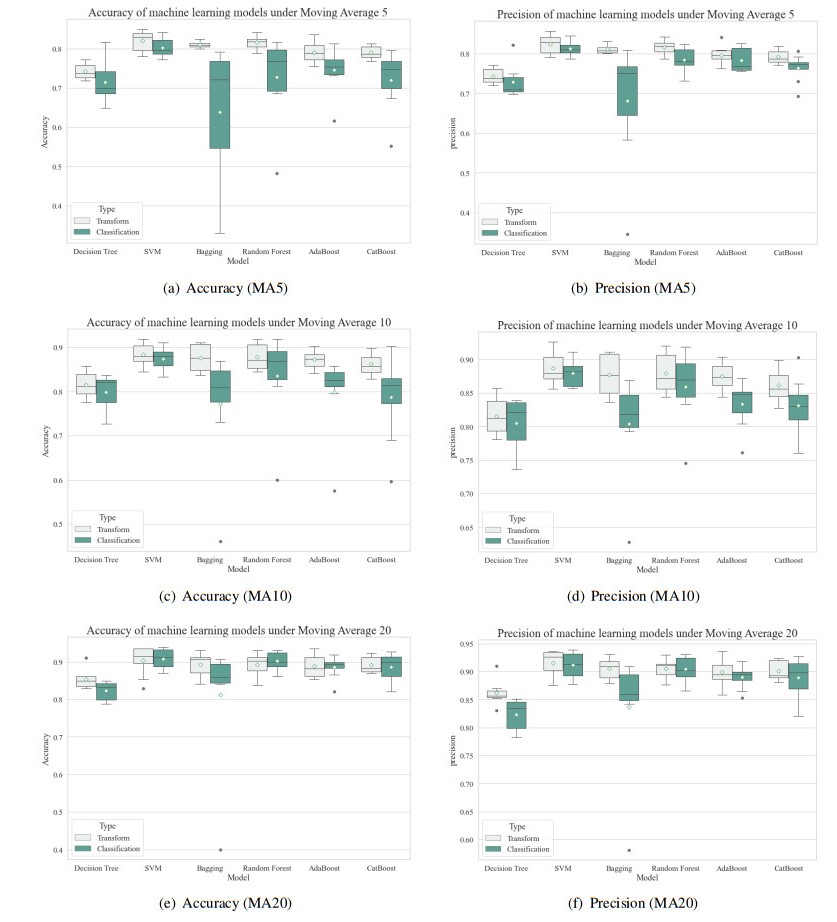
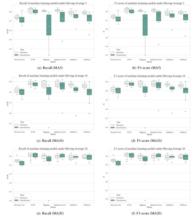
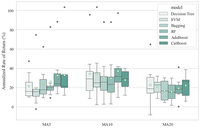
Stocks are the most common financial investment products and attract many investors around the world. However, stock price volatility is usually uncontrollable and unpredictable for the individual investor. This research aims to apply different machine learning models to capture the stock price trends from the perspective of individual investors. We consider six traditional machine learning models for prediction: decision tree, support vector machine, bootstrap aggregating, random forest, adaptive boosting, and categorical boosting. Moreover, we propose a framework that uses regression models to obtain predicted values of different moving average changes and converts them into classification problems to generate final predictive results. With this method, we achieve the best average accuracy of 0.9031 from the 20-day change of moving average based on the support vector machine model. Furthermore, we conduct simulation trading experiments to evaluate the performance of this predictive framework and obtain the highest average annualized rate of return of 29.57%.
Citation: Yimeng Wang, Keyue Yan. Machine learning-based quantitative trading strategies across different time intervals in the American market[J]. Quantitative Finance and Economics, 2023, 7(4): 569-594. doi: 10.3934/QFE.2023028
Stocks are the most common financial investment products and attract many investors around the world. However, stock price volatility is usually uncontrollable and unpredictable for the individual investor. This research aims to apply different machine learning models to capture the stock price trends from the perspective of individual investors. We consider six traditional machine learning models for prediction: decision tree, support vector machine, bootstrap aggregating, random forest, adaptive boosting, and categorical boosting. Moreover, we propose a framework that uses regression models to obtain predicted values of different moving average changes and converts them into classification problems to generate final predictive results. With this method, we achieve the best average accuracy of 0.9031 from the 20-day change of moving average based on the support vector machine model. Furthermore, we conduct simulation trading experiments to evaluate the performance of this predictive framework and obtain the highest average annualized rate of return of 29.57%.

| [1] |
Ampomah EK, Qin Z, Nyame G, et al. (2021) Stock market decision support modeling with tree-based AdaBoost ensemble machine learning models. Informatica 44. https://doi.org/10.31449/inf.v44i4.3159 doi: 10.31449/inf.v44i4.3159

|
| [2] |
Basak S, Kar S, Saha S, et al. (2019) Predicting the direction of stock market prices using tree-based classifiers. N Am J Econ Financ 47: 552–567. https://doi.org/10.1016/j.najef.2018.06.013 doi: 10.1016/j.najef.2018.06.013
|
| [3] | Breiman L (1996) Bagging predictors. Mach Learn 24: 123–140. |
| [4] | Breiman L (2001) Random forests. Mach Learn 45: 5–32. |
| [5] | Collobert R, Bengio S (2001) SVMTorch: Support vector machines for large-scale regression problems. J Mach Learn Res 1: 143–160. |
| [6] | Dinesh S, Rao N, Anusha SP, et al. (2021) Prediction of Trends in Stock Market using Moving Averages and Machine Learning. the 6th International Conference for Convergence in Technology: 1–5. https://doi.org/10.1109/I2CT51068.2021.9418097 |
| [7] |
Freund Y, Schapire RE (1997) A decision-theoretic generalization of on-line learning and an application to boosting. J Comput System Sci 55: 119–139. https://doi.org/10.1006/jcss.1997.1504 doi: 10.1006/jcss.1997.1504
|
| [8] | Géron A (2022) Hands-on machine learning with Scikit-Learn, Keras, and TensorFlow. O'Reilly Media, Inc. |
| [9] |
Henrique BM, Sobreiro VA, Kimura H (2018) Stock price prediction using support vector regression on daily and up to the minute prices. J Financ Data Sci 4: 183–201. https://doi.org/10.1016/j.jfds.2018.04.003 doi: 10.1016/j.jfds.2018.04.003
|
| [10] | Hindrayani KM, Fahrudin TM, Aji RP, et al. (2020) Indonesian stock price prediction including covid19 era using decision tree regression. the 3rd International Seminar on Research of Information Technology and Intelligent Systems: 344–347. https://doi.org/10.1109/ISRITI51436.2020.9315484 |
| [11] |
Kamalov F (2020) Forecasting significant stock price changes using neural networks. Neural Comput Appl 32: 17655-017667. https://doi.org/10.1007/s00521-020-04942-3 doi: 10.1007/s00521-020-04942-3
|
| [12] | Khaidem L, Saha S, Dey SR (2016) Predicting the direction of stock market prices using random forest. arXiv preprint: 1605.00003. https://doi.org/10.48550/arXiv.1605.00003 |
| [13] |
Khan W, Ghazanfar MA, Azam MA, et al. (2022) Stock market prediction using machine learning classifiers and social media, news. J Amb Intel Hum Comp 13: 3433–3456. https://doi.org/10.1007/s12652-020-01839-w doi: 10.1007/s12652-020-01839-w
|
| [14] | Lai CY, Chen RC, Caraka RE (2019) Prediction stock price based on different index factors using LSTM. 2019 International conference on machine learning and cybernetics: 1–6. https://doi.org/10.1109/ICMLC48188.2019.8949162 |
| [15] |
Li Y, Yan K (2023) Prediction of Barrier Option Price Based on Antithetic Monte Carlo and Machine Learning Methods. Cloud Comput Data Sci 4: 77–86. https://doi.org/10.37256/ccds.4120232110 doi: 10.37256/ccds.4120232110
|
| [16] |
Liu C, Wang J, Xiao D, et al. (2016) Forecasting S & P 500 stock index using statistical learning models. Open J Stat 6: 1067–1075. https://doi.org/10.4236/ojs.2016.66086 doi: 10.4236/ojs.2016.66086
|
| [17] |
Liu T, Ma X, Li S, et al. (2021) A stock price prediction method based on meta-learning and variational mode decomposition. Knowledge-Based Syst 252: 109324. https://doi.org/10.1016/j.knosys.2022.109324 doi: 10.1016/j.knosys.2022.109324
|
| [18] |
Nti IK, Adekoya AF, Weyori BA (2020) A systematic review of fundamental and technical analysis of stock market predictions. Artif Intell Rev 53: 3007–3057. https://doi.org/10.1007/s10462-019-09754-z doi: 10.1007/s10462-019-09754-z
|
| [19] | Obthong M, Tantisantiwong N, Jeamwatthanachai W, et al. (2020) A survey on machine learning for stock price prediction: Algorithms and techniques. Available from: https://eprints.soton.ac.uk/437785/ |
| [20] | Prokhorenkova L, Gusev G, Vorobev A, et al. (2018) CatBoost: unbiased boosting with categorical features. Adv Neural Inform Proc Syst 31. |
| [21] |
Subasi A, Amir F, Bagedo K, et al. (2021) Stock Market Prediction Using Machine Learning. Procedia Comput Sci 194: 173–179. https://doi.org/10.1016/j.procs.2021.10.071 doi: 10.1016/j.procs.2021.10.071
|
| [22] |
Vijh M, Chandola D, Tikkiwal VA, et al. (2020) Stock closing price prediction using machine learning techniques. Procedia Comput Sci 167: 599–606. https://doi.org/10.1016/j.procs.2020.03.326 doi: 10.1016/j.procs.2020.03.326
|
| [23] | Wang Y (2023) A study on stock price prediction based on machine learning models. Master dissertation, University of Macau: 1–56. |
| [24] | Wang Y, Yan K (2022) Prediction of Significant Bitcoin Price Changes Based on Deep Learning. 5th International Conference on Data Science and Information Technology (DSIT): 1–5. https://doi.org/10.1109/DSIT55514.2022.9943971 |
| [25] |
Wang Y, Yan K (2023) Application of Traditional Machine Learning Models for Quantitative Trading of Bitcoin. Artif Intell Evol 4: 34–48. https://doi.org/10.37256/aie.4120232226 doi: 10.37256/aie.4120232226
|
| [26] |
Yan K, Wang Y (2023) Prediction of Bitcoin prices' trends with ensemble learning models. 5th International Conference on Computer Information Science and Artificial Intelligence 12566: 900–905. https://doi.org/10.1117/12.2667793 doi: 10.1117/12.2667793
|
| [27] |
Yan K, Wang Y, Li Y (2023) Enhanced Bollinger Band Stock Quantitative Trading Strategy Based on Random Forest. Artif Intell Evol 4: 22–33. https://doi.org/10.37256/aie.4120231991 doi: 10.37256/aie.4120231991
|
| [28] | Zhang C, Ji Z, Zhang J, et al. (2018) Predicting Chinese stock market price trend using machine learning approach. the 2nd International Conference on Computer Science and Application Engineering: 1–5. https://doi.org/10.1145/3207677.3277966 |
| [29] |
Zhang J, Ye L, Lai Y (2023) Stock Price Prediction Using CNN-BiLSTM-Attention Model. Mathematics 11: 1985. https://doi.org/10.3390/math11091985 doi: 10.3390/math11091985
|
Figures(12) / Tables(14)

Yimeng Wang, Keyue Yan. Machine learning-based quantitative trading strategies across different time intervals in the American market[J]. Quantitative Finance and Economics, 2023, 7(4): 569-594. doi: 10.3934/QFE.2023028


 DownLoad: